How to Fix Hidden Rows in Excel (4 Effective Solutions)

Dataset Overview

Let’s delve into various solutions to address the issue of being unable to unhide rows in Excel. For our demonstration, we’ll work with a dataset representing sales data across different city branches in a super shop.

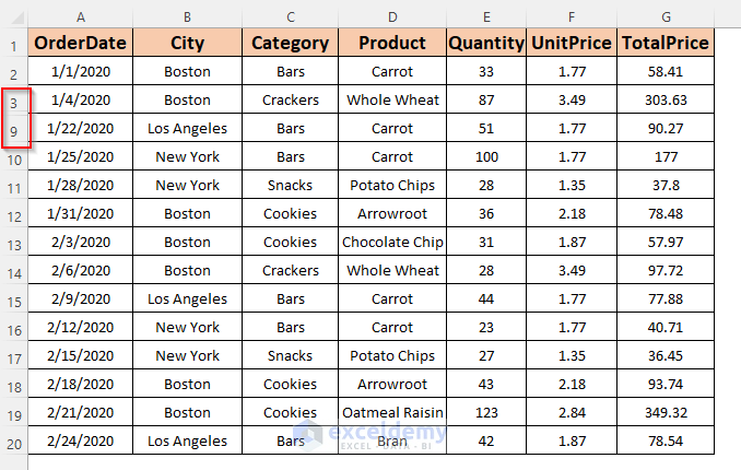
Solution 1 – Verify Row Height to Unhide Rows in Excel

In certain situations, rows may have such small heights that they become difficult to notice. Unfortunately, the standard methods for unhiding rows may not be effective in these cases. Let’s explore various scenarios related to row height.

Scenario 1: Row Height <= .07

For rows with a height of 0.07 or less, you can unhide them using any straightforward method.

Scenario 2:  .08 < Row Height < .67

Steps:

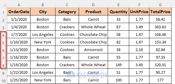
• Identify the hidden rows within your dataset. In this specific example, we’re dealing with rows 3 to 9.
• To select these hidden rows, follow these steps:
  • Click and drag your mouse cursor over the row numbers corresponding to rows 3 through 9. This action should highlight the entire range of rows.
  • Alternatively, you can hold down the Shift key and click on the row numbers individually to select them one by one.

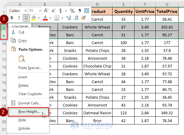
• Right-click on the selected rows or go to the Format tab in the Excel ribbon and choose Row Height.
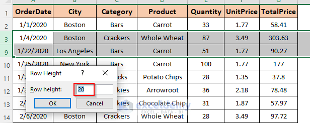
• Enter the visible number you want for the row height. For example, if you want a height of 20, type 20 into the box.
• Click the OK button to confirm your selection.

• Row Selection: Highlight rows 3 to 9. Note that rows 4 to 8 are currently hidden.
• Right-click to open the Context Menu.
• From the Context Menu, select the Unhide.

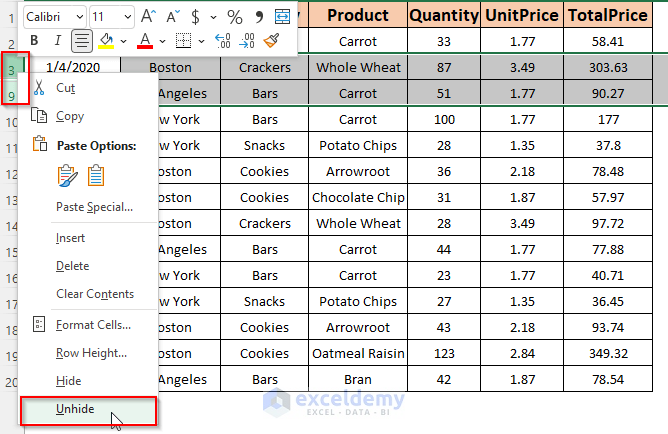
• These steps will reveal the hidden rows (4 to 8) and make them visible again.

Read More: VBA to Hide Rows Based on Cell Value in Excel

Solution 2 – Unfreezing Panes to Unhide Rows in Excel

Often, we utilize the freeze panes feature in Excel to navigate large datasets more efficiently. Imagine a scenario where the worksheet is scrolled upward, causing some rows to be out of view. In the screenshot below, the first 6 rows are hidden from sight:

When we use the Freeze Panes feature, it conceals those 6 rows.

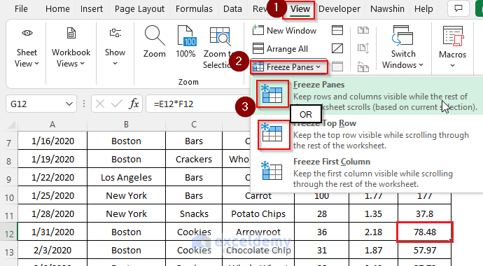
• Go to the View tab in the Excel Ribbon.
• Click on Freeze Panes.
• Choose either Freeze Panes or Freeze Top Row.

The only way to address this issue is by unfreezing the panes, which will make all the rows visible again. Follow these steps:

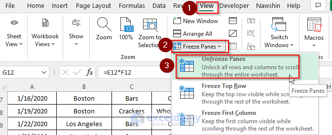
• Click on the View tab located in the Excel Ribbon.
• Within the View tab, locate the Freeze Panes
• Click on Unfreeze Panes to unlock all the rows that were previously hidden.

By following these steps, you’ll regain access to the rows that were concealed.

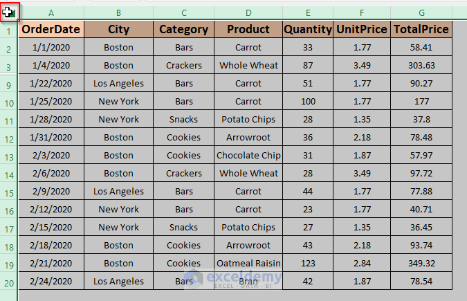
• Click the button located at the top left corner of the spreadsheet to select all cells.

• Navigate to the Format tab within the Home
• Select the Unhide Rows option from the Hide & Unhide

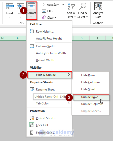
• Now, the previously hidden rows are visible.

Read More: How to Unhide Rows in Excel

Solution 3 – Deactivate the filter feature to unhide hidden rows in Excel

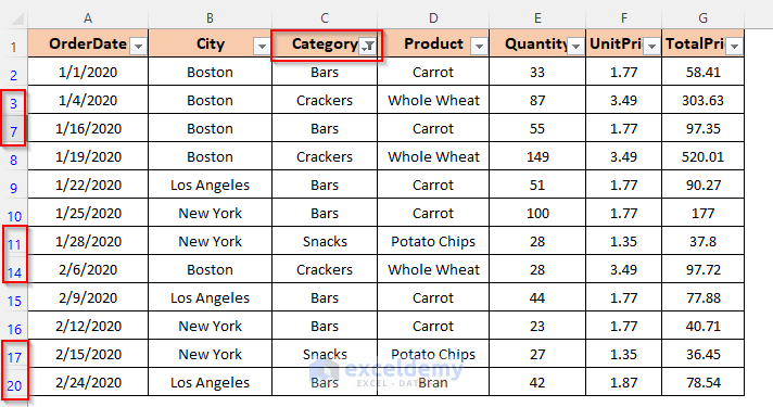
When we apply a filter to a dataset, it conceals the rows that do not meet the filter criteria. In the screenshot below, you’ll notice that rows 4-6, 12-13, and 18-19 have been hidden. The displayed products in the dataset are specifically filtered for the Bars, Crackers, and Snacks categories.

The dataset below outlines the filtering criteria applied to the previous dataset. Specifically, products categorized as Cookies have been hidden.

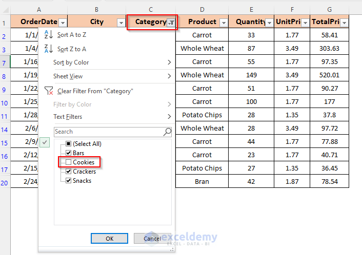
Unfortunately, conventional methods won’t allow us to unhide them.

To reveal the hidden rows, we need to deactivate the filter feature. Follow these steps:

• Navigate to the Data tab in the Excel Ribbon.
• Click on the Filter tab to deactivate the filter.

Alternatively, you can make the hidden rows visible by clicking on Select All.

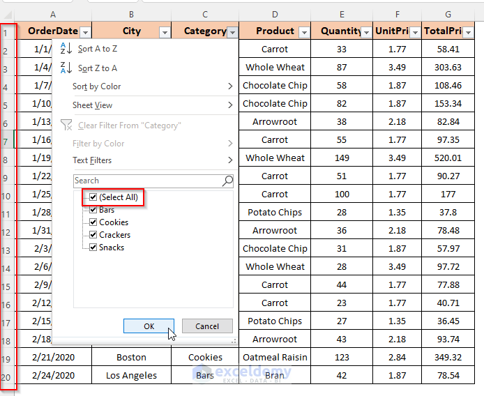
Read More: How to Unhide Top Rows in Excel

Solution 4 – Unhiding Hidden Rows in Excel by Double-Clicking the Double Line

If rows in a dataset are hidden due to either row height adjustments or filtering, there’s another clever trick to reveal them. Let’s walk through the steps:

• Look for a double line where the rows are hidden.
• By double-clicking this line, you can unhide the previously concealed rows.

• Hover your cursor over the double line where rows are hidden.

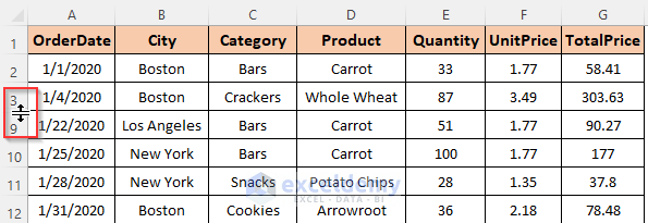
• Double-click once to reveal row 8.

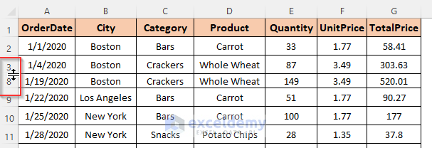
• Continue clicking the double line to unhide all the remaining hidden rows.

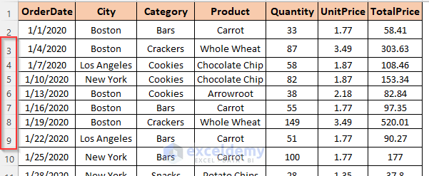
Read More: Unhide All Rows Not Working in Excel

Things to Remember

Ensuring that the worksheet is not protected is essential before applying any of the described methods. Once you’ve confirmed that, feel free to follow the steps provided to unhide hidden rows.

Download Practice Workbook

You can download the practice workbook from here:

Related Articles

• [Fixed!] Excel Rows Not Showing but Not Hidden
• Shortcut to Unhide Rows in Excel

<< Go Back to Hide Rows | Rows in Excel | Learn Excel