How to View All Sheets in Excel at Once (5 Easy Ways)

Method 1 – Viewing Two Sheets from the Same Workbook Side by Side

Steps:

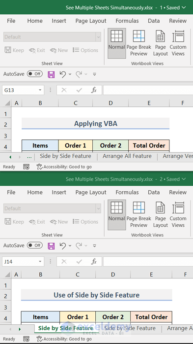
• Click on the View tab.
• In the Window group, click on New Window.

• Also in the Window group, click on View Side by Side.

• Select the sheet you want to compare by clicking it in each workbook window.

The sheets open in the default horizontal layout.

Method 2 – Viewing Two Sheets from Different Excel Workbooks Side by Side

Steps:

• Open both the workbooks containing the worksheets you want to compare.
• Click on the View tab.
• In the Window group, select View Side by Side.

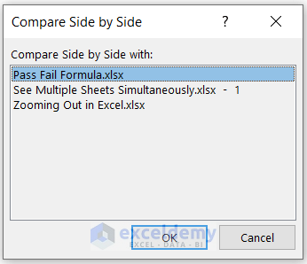
• When there are more than two open worksheets, the Compare Side by Side dialog box opens.
• Click the workbook that includes the worksheet that you want to compare with your active worksheet.
• Click OK.

• Click the sheet you want to compare in each workbook window.

The sheets open in the default horizontal layout.

Method 3 – Using Arrange All to Arrange Multiple Sheets Vertically at Once

Excel’s Arrange All feature can be used to configure viewing sheets from multiple workbooks in different layouts.

Steps:

• Open all required workbooks.
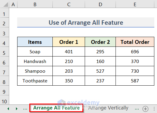
• Click the desired sheet tab.

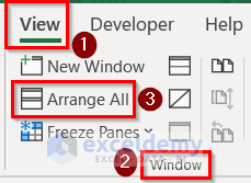
• Click the View tab.
• Select New Window from the Window group.

• Click on Arrange All in the Window group.

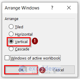
• A dialog box named Arrange Windows opens.
• Select Vertical from the Arrange section.
• Click OK to arrange the sheets vertically.

Method 4 – View All Sheets at Once by Right-Clicking

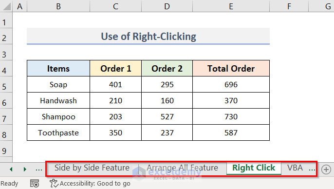
In an Excel file, the tabs for each sheet are located at the bottom. However, not all tabs can be displayed simultaneously when a document contains a lot of sheets. For example, there are 8 worksheets in the following example, but only 4 of them are visible. Here’s how to view all the sheets:

Steps:

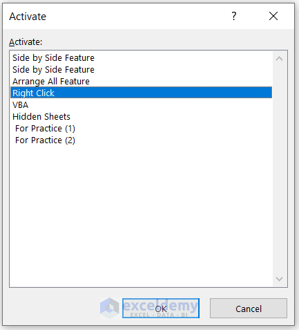
• Simply right-click the arrow located at the left of the sheet tabs to see the entire list of worksheets.

• A pop-up list named Activate showing the titles of every worksheet opens.
• Jump to any worksheet by selecting it from the list and clicking OK.

Method 5 – Applying VBA to List All Sheets at Once

In this method, we have used colors in the sheet tab, which will be visible in the generated list too.

Steps:

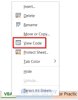
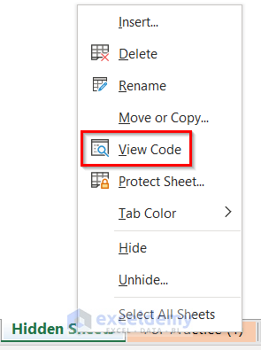
• Right-click a sheet from the sheet tab section at the bottom of the workbook.
• Select View Code from the drop-down.

• Microsoft Visual Basic for Applications window opens.
• Enter the below code in the Code window.
• In the 3rd row of the code, change “VBA” to the name of your sheet, if required.

Sub ApplyingVBA()
Dim RowNumber As Integer
Sheets("VBA").Select
RowNumber = 4
For Each Sheet In Application.Worksheets
Range("B" & RowNumber).Value = Sheet.Name
With Range("B" & RowNumber).Interior
.Pattern = xlSolid
.PatternColorIndex = xlAutomatic
.Color = Sheet.Tab.Color
.TintAndShade = 0
.PatternTintAndShade = 0
End With
RowNumber = RowNumber + 1
Next Sheet
End Sub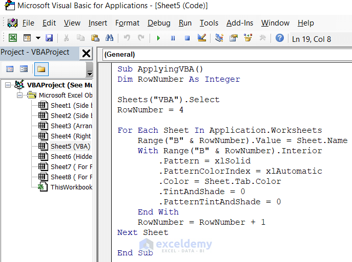

• Click the Run tab.
• Select RunSub/UserForm to run the VBA code.

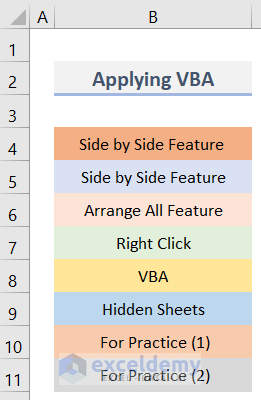
The list of all the Excel worksheets in the sheet is returned.

Moreover, the sheet names will retain the colors of their corresponding tabs.

How to View All Hidden Sheets at Once in Excel

The Immediate Window feature of VBA can be used view all hidden worksheets.

Steps:

• Right-click on any worksheet from the sheet tab section located at the bottom of your workbook.
• Click View Code.

• The Microsoft VBA window opens.
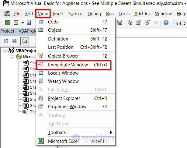
• Click View on the menu.
• Select Immediate Window from the drop-down.

• VBA Editor displays the Immediate window.
• Copy and paste the following code into the Immediate window:

For each Sheet in Thisworkbook.Sheets: Sheet.Visible=True: Next Sheet

• Most importantly, put the cursor where the line of the code ends.

• Press Enter.

All the hidden sheets of the Excel workbook are visible at once.

Download Practice Workbook

Related Article

• What Is Normal View in Excel?

<< Go Back to View in Excel | Learn Excel