Introduction to Fuzzy Match
A Fuzzy Match is a type of partial match.
In these types of matches, one text does not match fully to the other text. But the important sections of the text do match the other text.

In the given example, the book “The History of India during the World War” contains three important sections: History, India, and World War.
Therefore, all the books that contain either one or more than one of these sections will fuzzily match the book.
So, the fuzzy matches are:
- The History of the Second World War
- History of the Ancient Greece
- World War: Causes and Effects
- The Indus Civilization: An Ancient History
- India Wins Freedom
- Adolf Hitler: Before and After the World War
- The Discovery of India
VLOOKUP Fuzzy Match in Excel: 3 Approaches
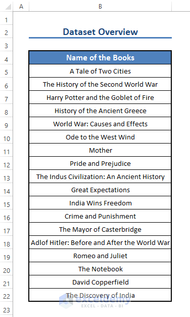
Here we’ve got a data set with the Names of some books. Our objective today is to use the VLOOKUP function of Excel to generate some Fuzzy Matches. Let’s discuss 3 different approaches.
Method 1 – VLOOKUP Fuzzy Match Using Wildcards (Entire Lookup_Value Matching)
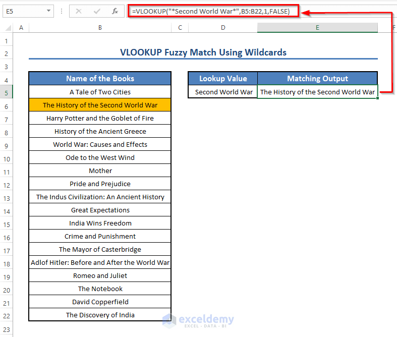
The wildcard character is the Asterisk (*) symbol. You have to match the entire lookup_value in this method, not the separate parts of the lookup_value. For example, we can find a book containing the text “Second World War” in this way, and only the books having the full text “Second World War” will match.
The formula will be:
=VLOOKUP("*Second World War*",B5:B22,1,FALSE)
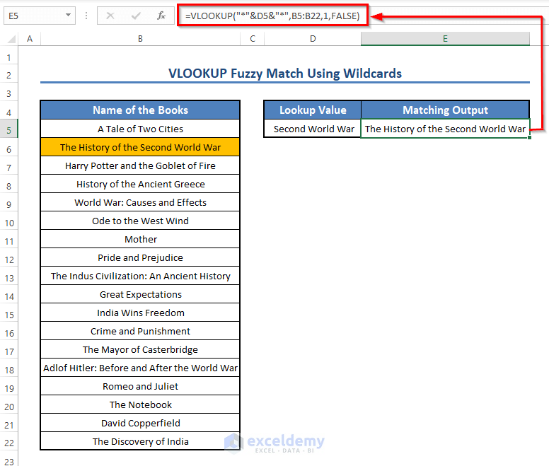
You can also use a cell reference in place of the original text. Use the Ampersand (&) symbol to merge them into a single text, like this:
=VLOOKUP("*"&D5&"*",B5:B22,1,FALSE)
To know more about VLOOKUP using wildcards, see this article.
Method 2 – Fuzzy Match Using VBA
- Open a VBA window and insert the following VBA code in a new module:
Code:
Function FUZZYMATCH(str As String, rng As Range)

str = LCase(str)

Dim Remove_1(5) As Variant
Remove_1(0) = ","
Remove_1(1) = "."
Remove_1(2) = ":"
Remove_1(3) = "-"
Remove_1(4) = ";"
Remove_1(5) = "?"

Dim Rem_Str_1 As String
Rem_Str_1 = str
Dim rem_count_1 As Variant

For Each rem_count_1 In Remove_1
    Rem_Str_1 = Replace(Rem_Str_1, rem_count_1, "")
Next rem_count_1

Words = Split(Rem_Str_1)

Dim i As Variant
For i = 0 To UBound(Words)
    If Len(Words(i)) = 1 Or Len(Words(i)) = 2 Then
        Words(i) = Replace(Words(i), Words(i), " bt ")
    End If
Next i

Dim Final_Remove(26) As Variant
Final_Remove(0) = "the"
Final_Remove(1) = "and"
Final_Remove(2) = "but"
Final_Remove(3) = "with"
Final_Remove(4) = "into"
Final_Remove(5) = "before"
Final_Remove(6) = "after"
Final_Remove(7) = "beyond"
Final_Remove(8) = "here"
Final_Remove(9) = "there"
Final_Remove(10) = "his"
Final_Remove(11) = "her"
Final_Remove(12) = "him"
Final_Remove(13) = "can"
Final_Remove(14) = "could"
Final_Remove(15) = "may"
Final_Remove(16) = "might"
Final_Remove(17) = "shall"
Final_Remove(18) = "should"
Final_Remove(19) = "will"
Final_Remove(20) = "would"
Final_Remove(21) = "this"
Final_Remove(22) = "that"
Final_Remove(23) = "have"
Final_Remove(24) = "has"
Final_Remove(25) = "had"
Final_Remove(26) = "during"

Dim w As Variant
Dim ww As Variant
For w = 0 To UBound(Words)
    For Each ww In Final_Remove
        If Words(w) = ww Then
            Words(w) = Replace(Words(w), Words(w), " bt ")
            Exit For '
        End If
    Next ww
Next w
Dim Lookup As Variant
Dim x As Integer
x = rng.Rows.count
ReDim Lookup(x - 1)
Dim j As Variant
j = 0
Dim k As Variant
For Each k In rng
    Lookup(j) = k
    j = j + 1
Next k

Dim Lower As Variant
ReDim Lower(UBound(Lookup))
Dim u As Variant
For u = 0 To UBound(Lookup)
    Lower(u) = LCase(Lookup(u))
Next u

Dim out As Variant
ReDim out(UBound(Lookup), 0)

Dim count As Integer
co = 0
mark = 0
Dim m As Variant
For m = 0 To UBound(Lower)
    Dim n As Variant
    For Each n In Words
        Dim o As Variant
        For o = 1 To Len(Lower(m))
            If Mid(Lower(m), o, Len(n)) = n Then
                out(co, 0) = Lookup(m)
                co = co + 1
                mark = mark + 1
                Exit For
            End If
        Next o
        If mark > 0 Then
            Exit For
        End If
    Next n
    mark = 0
Next m

Dim output As Variant
ReDim output(co - 1, 0)
Dim z As Variant
For z = 0 To co - 1
    output(z, 0) = out(z, 0)
Next z

FUZZYMATCH = output

End Function
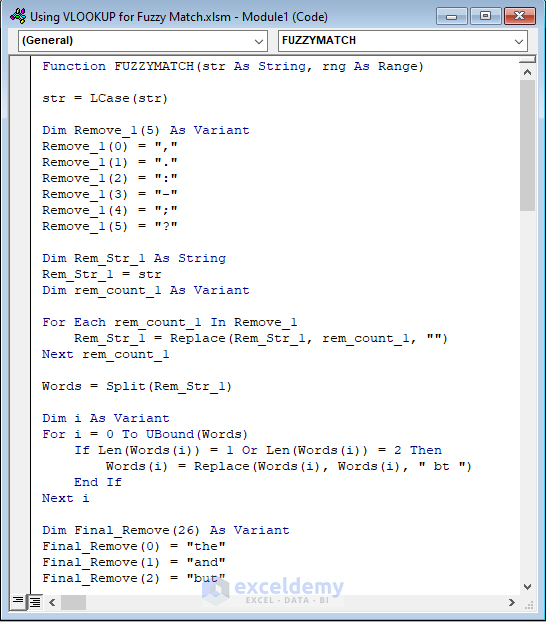
This code builds a function called FUZZYMATCH.
- Save the code (you can use the steps of Method 3 of this article).
This FUZZYMATCH function finds out all the Fuzzy Matches of a Lookup Value directly.
The Syntax of this FUZZYMATCH function is:
=FUZZYMATCH(lookup_value,lookup_range)
To find out the Fuzzy Matches of the book “The History of India during the World War”, enter this lookup_value in a cell (D5 in this example) and enter this formula in another cell:
=FUZZYMATCH(D5,B5:B22)
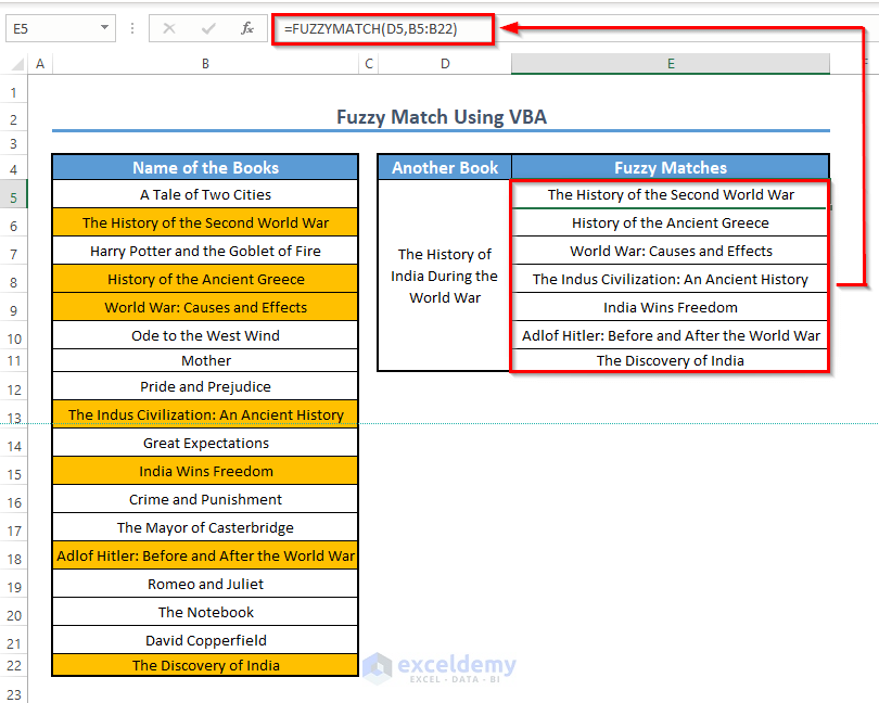
See, we have found all the Fuzzy Matches in the book “The History of India during the World War.” Here, D5 is the cell reference of the lookup_value (“The History of India during the World War”), and B5:B22 is the lookup_range.
Let’s find out the Fuzzy Matches of another book called “A Notebook of the Causes behind the Crime of Big Cities”.
- Enter this lookup_value in a cell (D5 in this example) and enter this formula in another cell:
=FUZZYMATCH(D5,B5:B22)
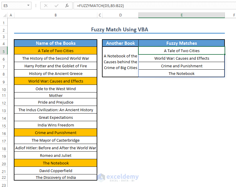
💡 Explanation of Formula
- The FUZZYMATCH function is the function we built in VBA. It takes a string called lookup_value and a range of cells called lookup_range and returns an array of all the Fuzzy Matches of the string.
- Therefore FUZZYMATCH(D5,B5:B22) returns an array of all the Fuzzy Matches of the string in cell D5 from the range B5:B22.
Read More: VLOOKUP and Return All Matches in Excel
Method 3 – Fuzzy Match Using Fuzzy Lookup Add-in of Excel
- Download and install the Fuzzy Lookup Add-in
- You will find the Fuzzy Lookup Add-in in your Excel Toolbar.

- Arrange the dataset into two tables that you want to match.
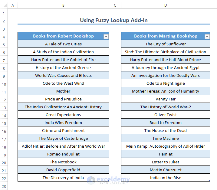
- We’ve got two tables containing two lists of books from two bookshops called Robert Bookshop and Marting Bookshop.
- Go to the Fuzzy Lookup tab and click on the Fuzzy Lookup tool in the Excel Toolbar.
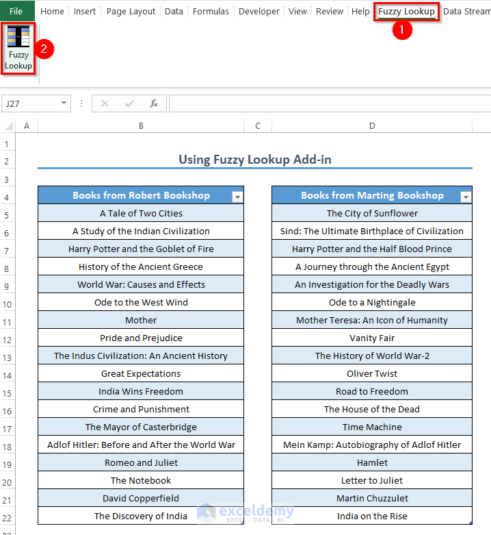
- You will get a Fuzzy Lookup table in the side panel of your workbook.
- In the Left Table and Right Table options, choose the names of the two tables. For this example, we chose Robert and Martin.
- In the Columns section, choose the names of the columns of each table.
- In the Match Column section, select the type of match that you want between the two columns. For Fuzzy Match, select Default.
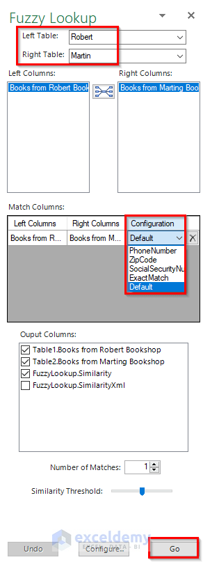
- Click on Go. You will get the matching ratio of the tables in a new table.
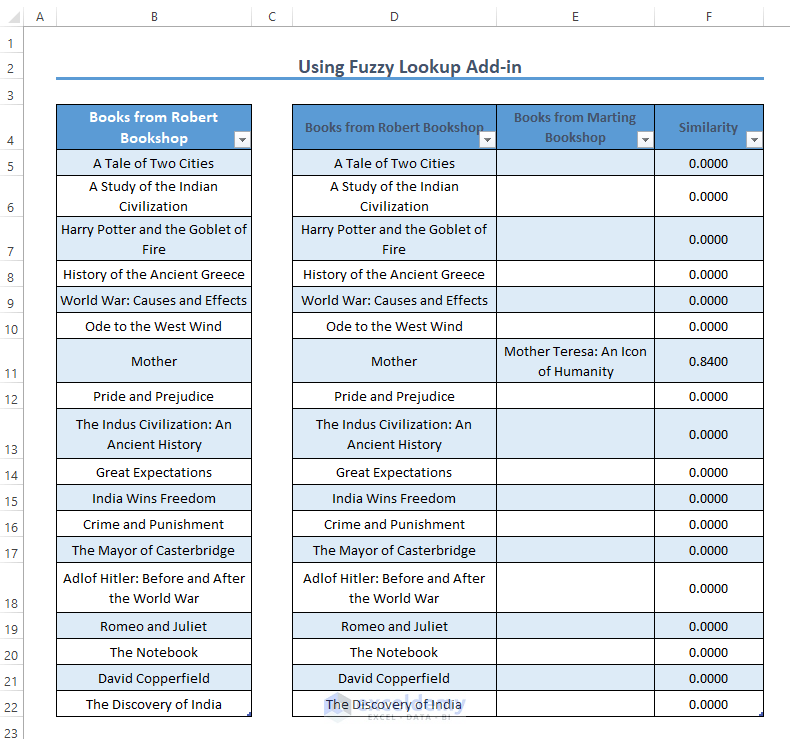
Read More:How to Use VLOOKUP Function with Exact Match in Excel
Download the Practice Workbook
Further Readings
- How to Use VLOOKUP with Two Lookup Values in Excel
- How to Apply Double VLOOKUP in Excel?
- How to Find Second Match with VLOOKUP in Excel
- Excel VLOOKUP to Find Last Value in Column
- How to Use VLOOKUP to Search Text in Excel
- How to Apply VLOOKUP by Date in Excel
- Return the Highest Value Using VLOOKUP Function in Excel
- VLOOKUP with Numbers in Excel
<< Go Back to Advanced VLOOKUP | Excel VLOOKUP Function | Excel Functions | Learn Excel
Get FREE Advanced Excel Exercises with Solutions!

