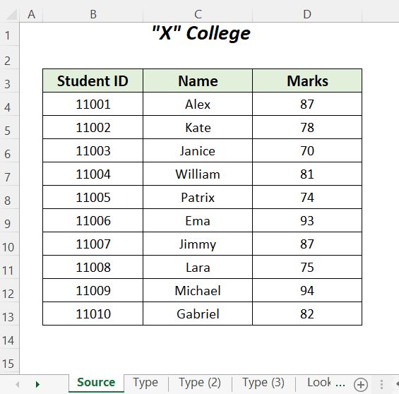
This is the Source sheet from which you will extract data.
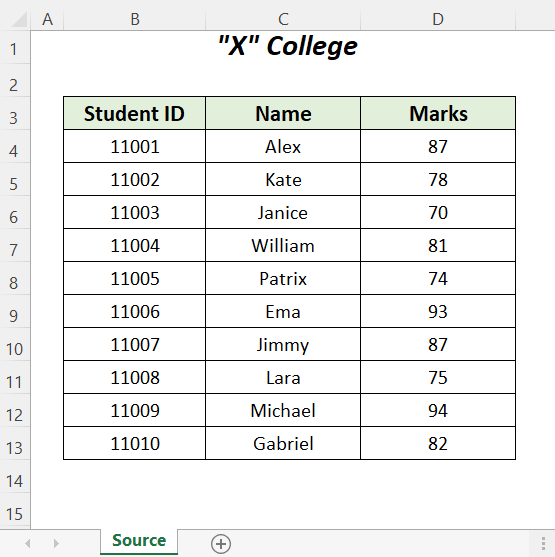
Solution 1- Entering the Correct Lookup Value, the Worksheet Name, and the Column Index Number
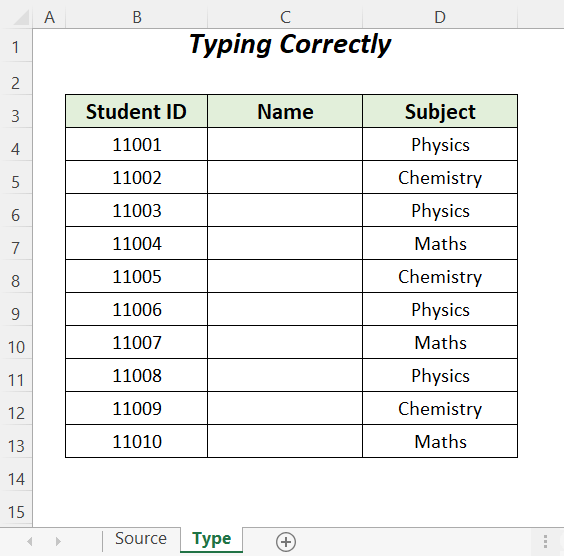
In a new worksheet (Type), extract the names corresponding to the Student ID numbers in the Source worksheet.
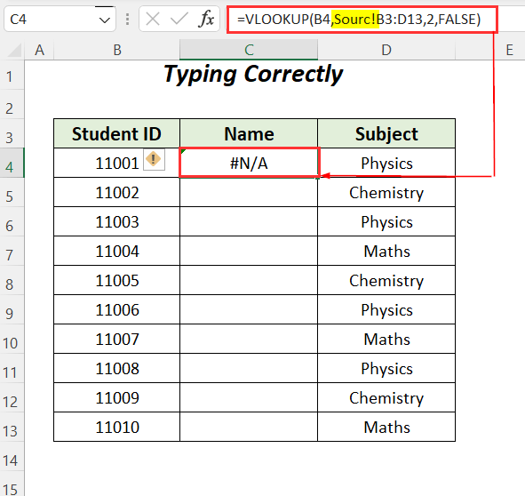
- The name of the worksheet is misspelled: Sourc and the #N/A error is displayed.
- Enter the following formula with the correct sheet name.
=VLOOKUP(B4,Source!$B$3:$C$13,2,FALSE)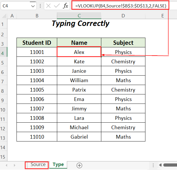
- Using a lookup value that does not match the values in the lookup array can also return a the #N/A error. Here, 1001, instead of 11001.
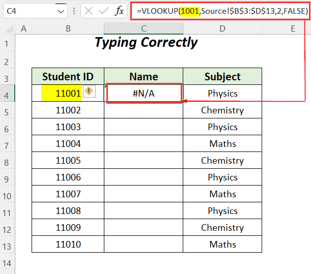
- Enter the correct lookup value. This is the formula.
=VLOOKUP(11001,Source!$B$3:$D$13,2,FALSE)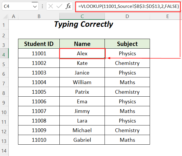
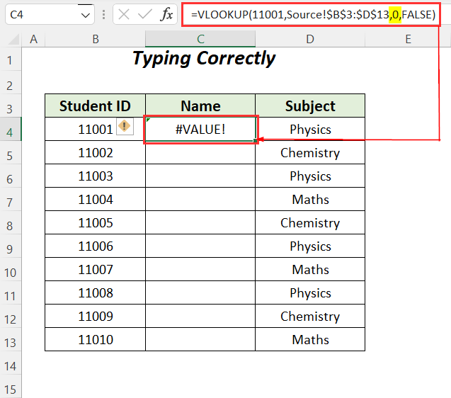
If the correct column index number isn’t provided, the #VALUE! error is displayed.
Here, column number was 2, but we 0 was the input.
- Use the following formula.
=VLOOKUP(11001,Source!$B$3:$D$13,2,FALSE)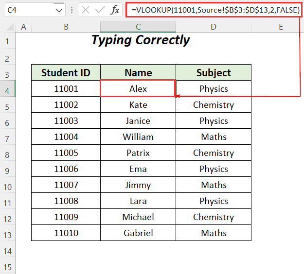
Solution 2 – Creating a Dataset with the Lookup Value in the First Column
In the Source dataset, the Name column is in the first position. If you look up any value in any other column, the VLOOKUP will not work between the sheets.
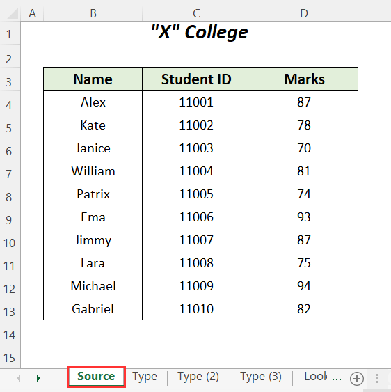
In the Lookup table serial datasheet, the students’ names were extracted depending on their ids.
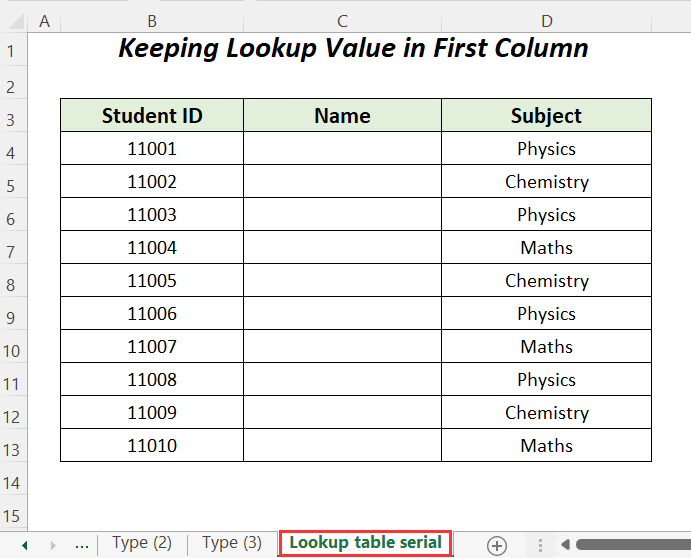
- Enter the following formula.
=VLOOKUP(B4,Source!B3:D13,1,FALSE)The output is showing an error because the value in B4 is not in the first column of the Source datasheet.
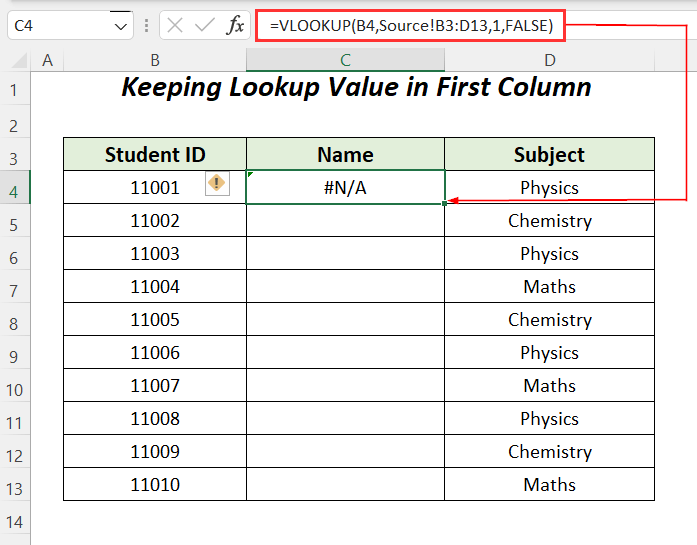
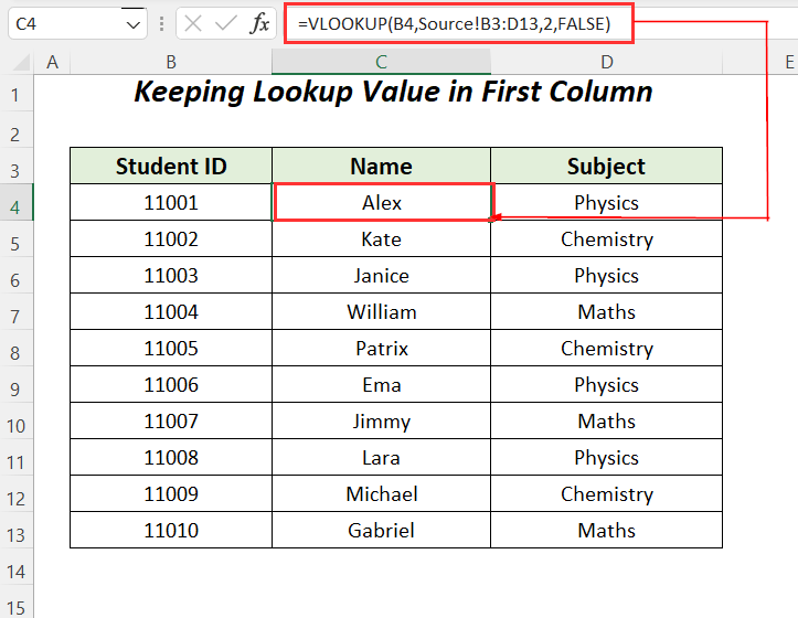
- Place Student ID in the first column, so that it contains the lookup value.
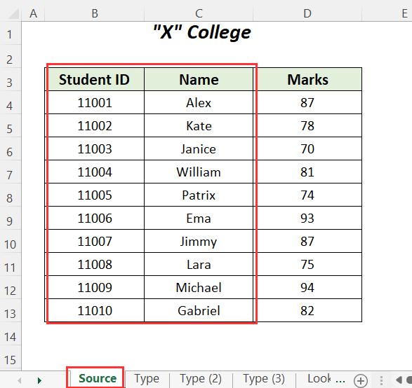
- Enter the following formula.
=VLOOKUP(B4,Source!B3:D13,2,FALSE)This is the output.
Solution 3 – Applying an Absolute Reference
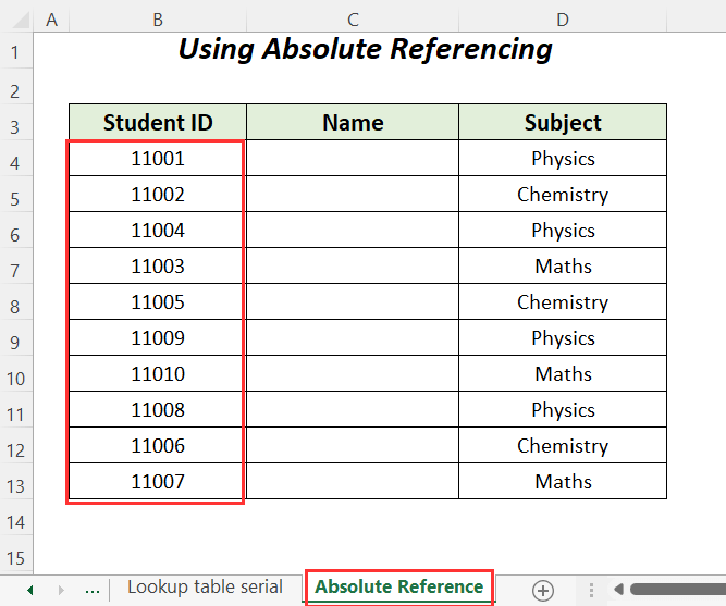
The serial numbers were changed in the Student ID column.
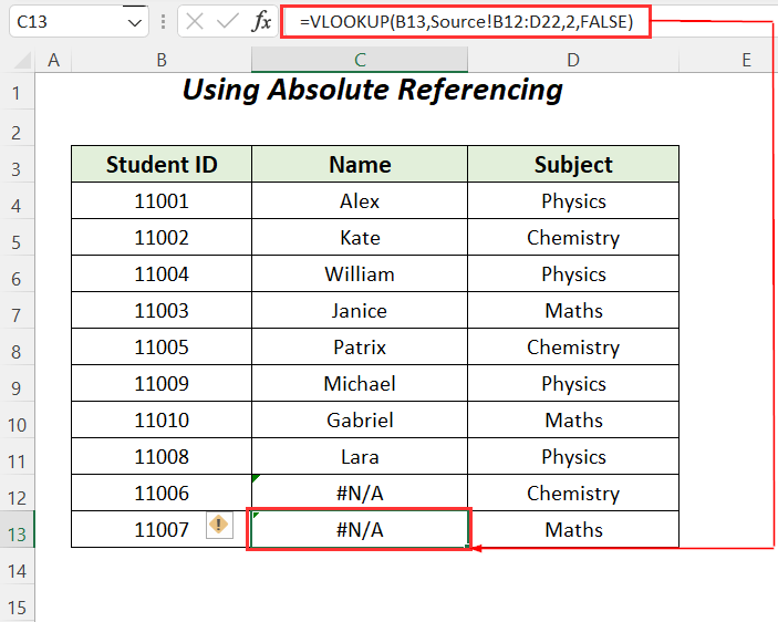
Using the formula like in the previous methods, the two last cells display errors and the reference of the main table array changed from B3:D13 to B12:D22.
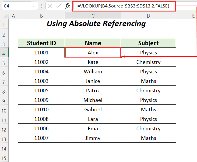
- Use the following formula with absolute referencing.
=VLOOKUP(B4,Source!$B$3:$D$13,2,FALSE)You will be able to extract the correct values from the Source worksheet.
Solution 4 – Cleaning Hidden Spaces in the Lookup Values
Sometimes there are hidden spaces or characters in the lookup array which can cause VLOOKUP not to work between sheets.
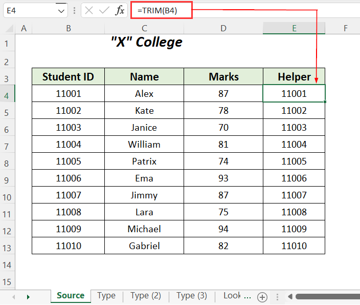
- Go to the Source sheet, add an extra column (Helper), and enter the following formula.
=TRIM(B4)The TRIM function will clear out extra spaces in the Student ID column.
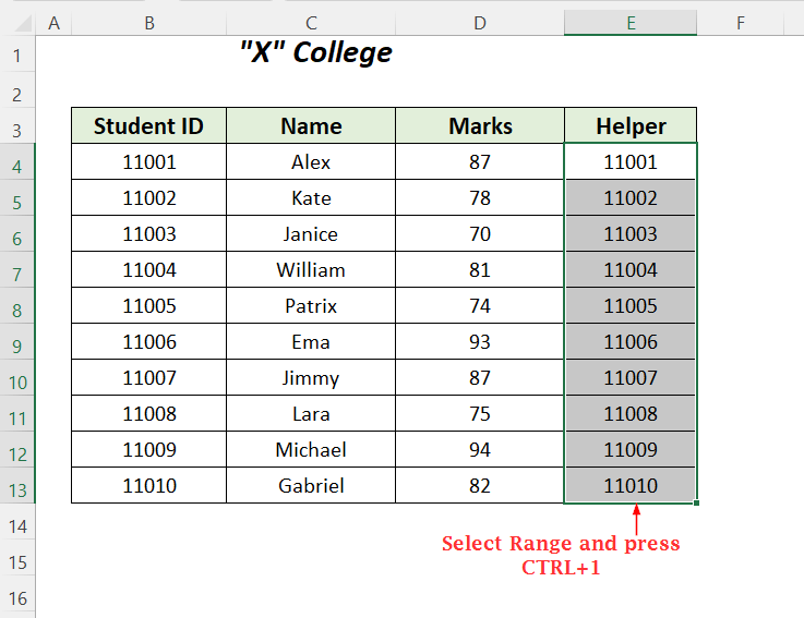
The numbers will be formatted as text. You must change their format to number.
- Select the range in the Helper column and press CTRL+1.
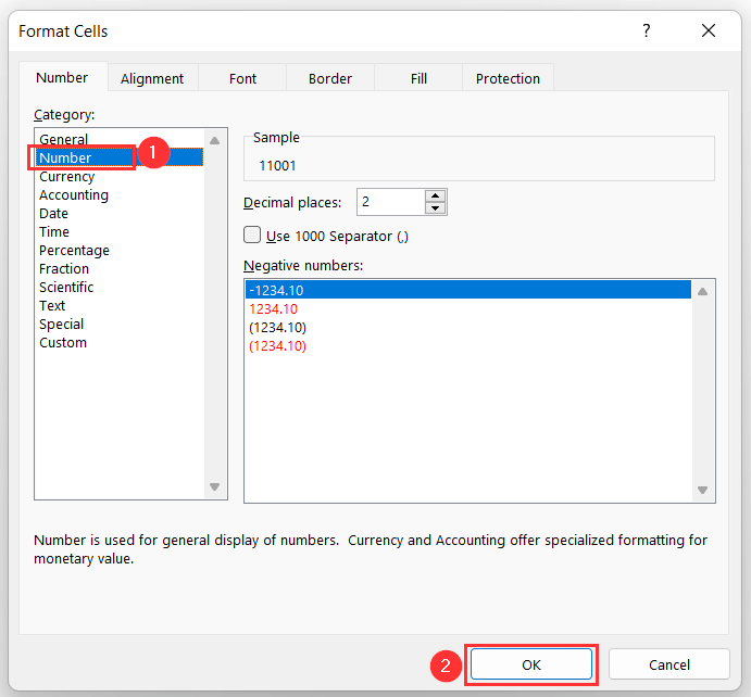
In the Format Cells dialog box:
- Choose the Category as Number and click OK.
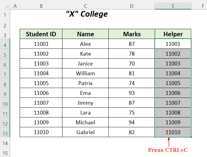
- Select the range and press CTRL+C to copy.
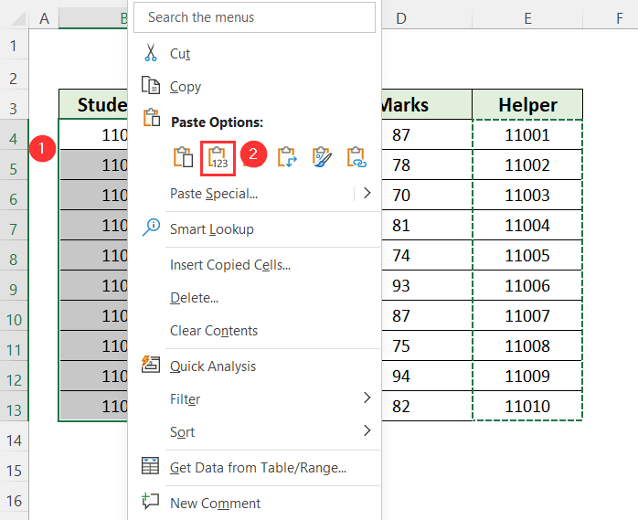
- Choose the main column Student ID, right-click it, and select Paste Values.
- You can delete the Helper column.
- Enter the following formula to get the results.
=VLOOKUP(B4,Source!$B$3:$D$13,2,FALSE)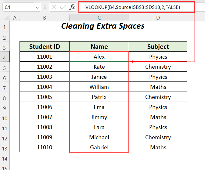
Solution 5 – Using a Lookup Value Greater Than the Smallest Value in the Array for an Approximate Match
A new ID: 11000 was inserted.
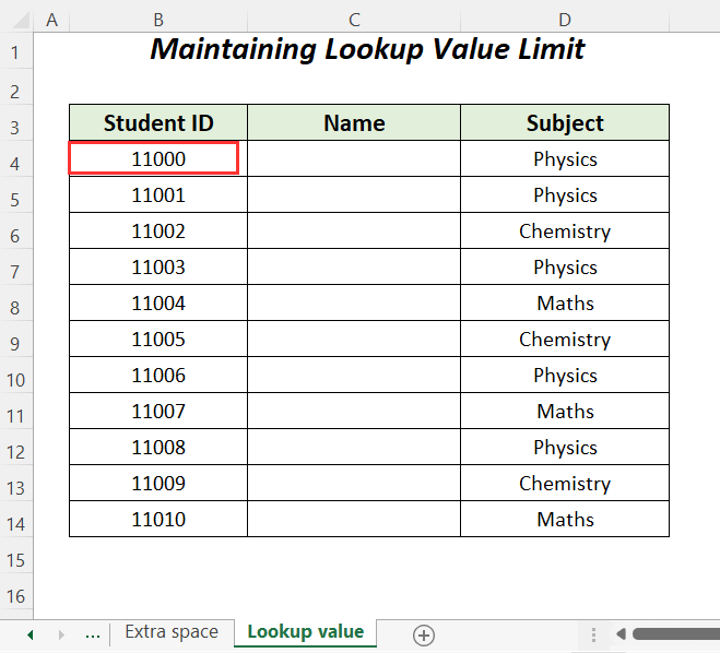
After using the following formula, the #N/A error is displayed.
=VLOOKUP(B4,Source!$B$3:$D$13,2,TRUE)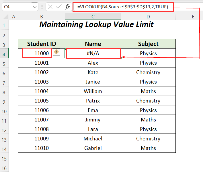
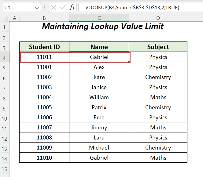
- Use the ID 11011 instead of 11000, and the error will be removed.
The VLOOKUP will work correctly between sheets and return an approximate value.
Solution 6 – Arranging Values in the Lookup Array in Ascending Order
The order of the dataset in the Source worksheet was changed into descending order.
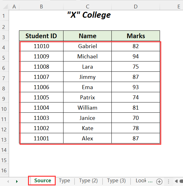
Because of the descending order, the formula returns the #N/A error.

Change the order of the dataset in the Source worksheet:
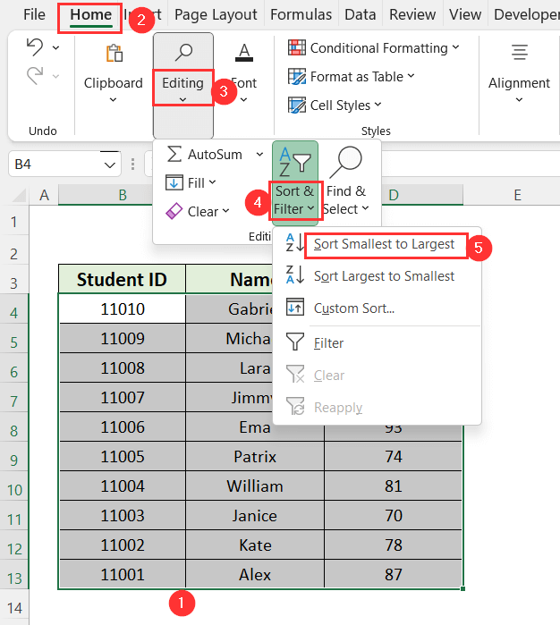
- Go to the Home tab >> Editing >> Sort & Filter >> Sort Smallest to Largest.
The dataset will be displayed in ascending order.
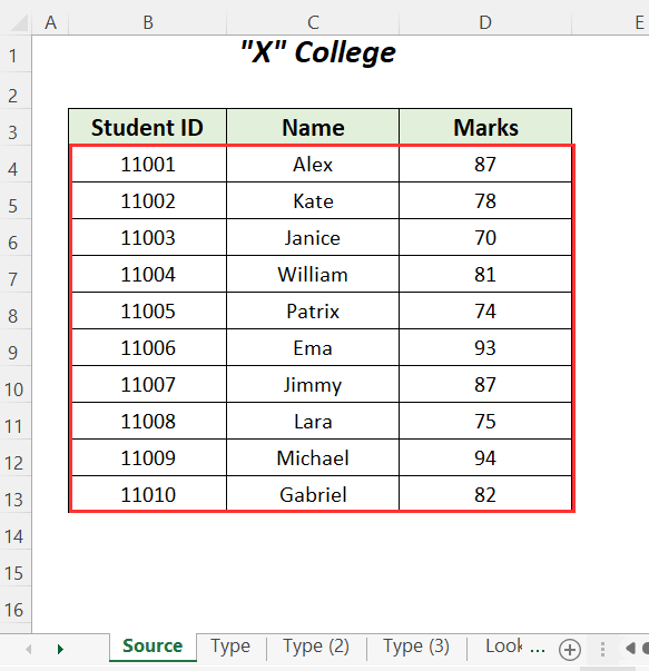
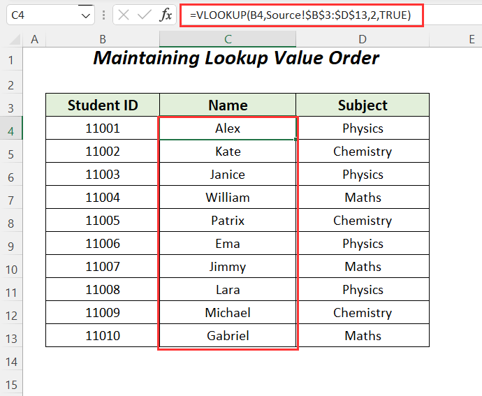
- Go to the worksheet from which you want to extract data.
This is the output.
Solution 7 – Checking If Numbers are Formatted as Numbers and Not Texts
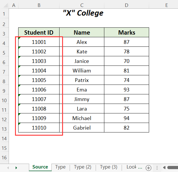
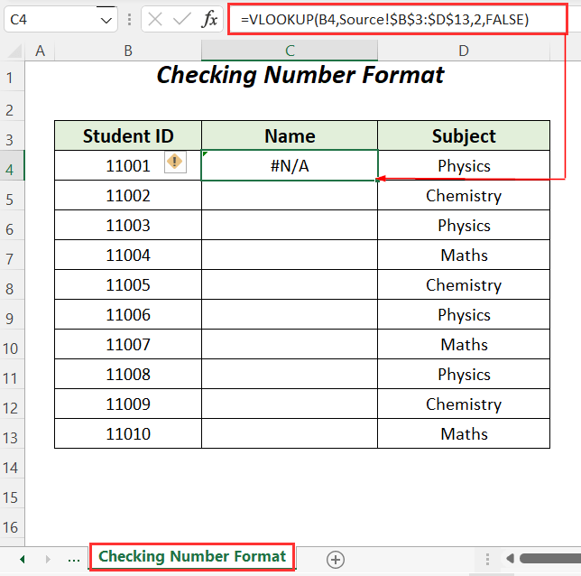
In the Source worksheet, numbers are stored as text.
- Use the following formula to extract names.
=VLOOKUP(B4,Source!$B$3:$D$13,2,FALSE)It will return an error.
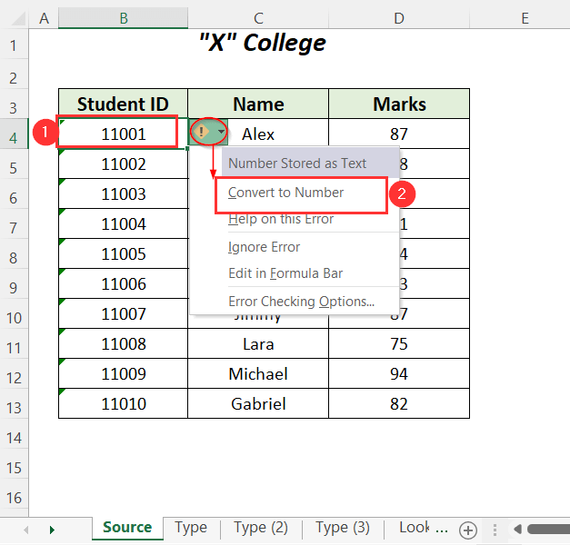
- Go to the Source worksheet, select the cell, click the error symbol, and choose Convert to Number.
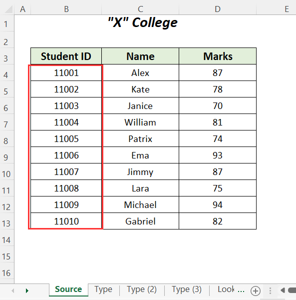
This is the output.
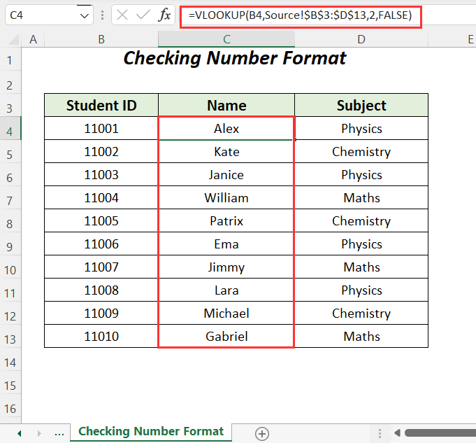
- Go to the sheet from which you want to extract values, and enter the following formula.
=VLOOKUP(B4,Source!$B$3:$D$13,2,FALSE)This is the output.
Read More: [Solved]: Excel VLOOKUP Not Working with Numbers
Solution 8 – Adjust the Formula after Inserting or Deleting A Column
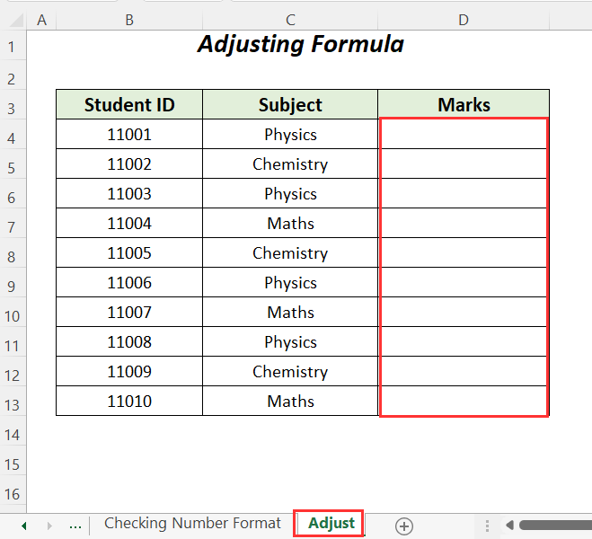
- Enter the following formula to get the results below.
=VLOOKUP(B4,Source!$B$3:$D$13,3,FALSE)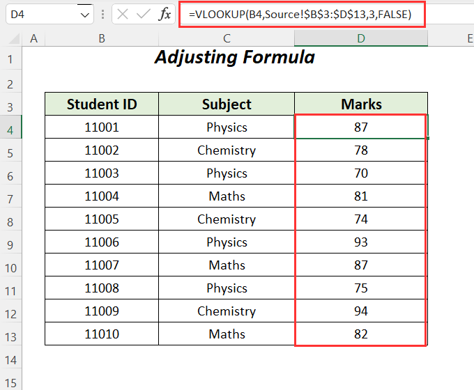
- Delete the Name column in the Source worksheet.
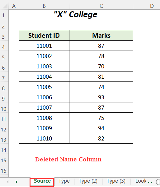
the #REF! error will be displayed due to the change of the index column number.
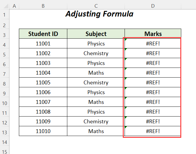
- Use the following formula.
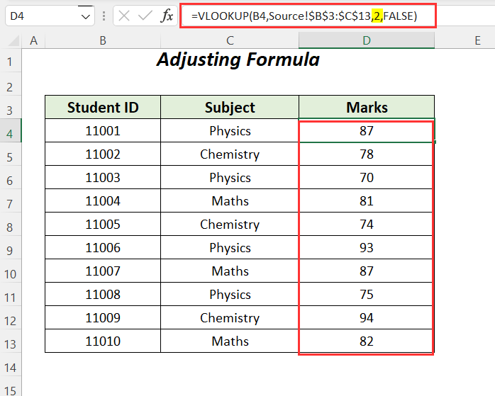
=VLOOKUP(B4,Source!$B$3:$C$13,2,FALSE)This is the output.
How to Fix it When the VLOOKUP Is Not Working Between Workbooks in Excel?
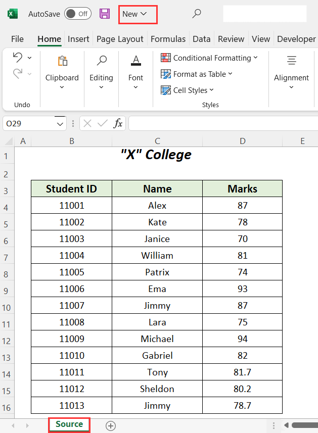
The main dataset is in the Source sheet of the New workbook.
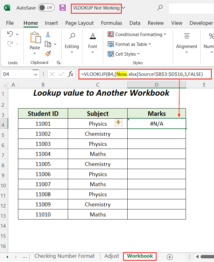
By entering Now instead of New (the workbook name) errors are displayed.
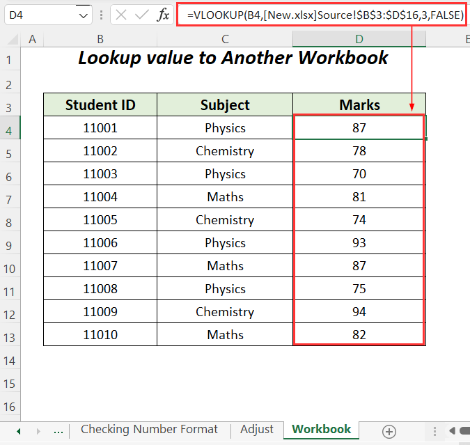
- Enter the following formula with the correct name.
=VLOOKUP(B4,[New.xlsx]Source!$B$3:$D$16,3,FALSE)This is the output.
Download Workbook
Related Articles
- [Fixed!] Excel VLOOKUP Not Working Due to Format
- [Fixed!] Excel VLOOKUP Drag Down Not Working
- VLOOKUP Not Picking up Table Array in Another Spreadsheet
<< Go Back to Issues with VLOOKUP | Excel VLOOKUP Function | Excel Functions | Learn Excel
Get FREE Advanced Excel Exercises with Solutions!


Hi
Thanks a lot for this detailed explanation.
However, it keeps giving #N/A also after checking everything!
Dear Ahmad,
Thanks for your query.
In the VLOOKUP function #N/A error occurs when you type the wrong lookup value or worksheet name. So, check if you have given the lookup value and worksheet name properly.
Again, VLOOKUP can only look up values to the right of the lookup value. Be careful about this.
If you need further help, please mention details about your problem.
Regards
Mahfuza Anika Era
ExcelDemy