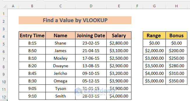
To demonstrate how to use VLOOKUP to find a value within a range, we’ll use the following dataset, which contains information about some Employees – their Names, Joining Date, Entry Time, Salary, and Bonus according to Salary Range.
Example 1 – Find a Bonus Within a Salary Range
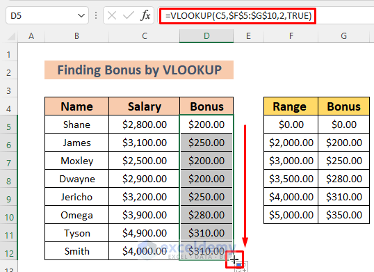
In the dataset, we set bonuses according to a salary range. For instance, those who have salaries in the range of $2000-2999 receive a bonus of $200; those who have salaries in the range of $3000-3499 receive a bonus of $250 and so on.
Let’s determine our Employees’ bonuses using the VLOOKUP Function.
Steps:
- First, we modify our dataset, as we don’t need the Entry Time and Joining Date in this section.
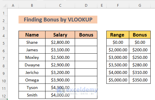
- Enter the following formula in cell D5:
=VLOOKUP(C5,$F$5:$G$10,2,TRUE)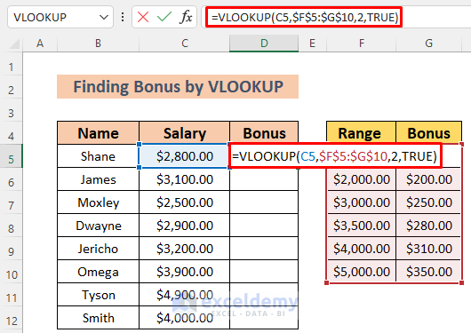
The VLOOKUP Function looks for the Salary in cell C5 within the range of F5:G10. As we want to determine Bonuses, which are in the 2nd column of F5:G10, we set 2 as the col_index_num. We’re looking for an approximate_match for the Salary in cell C5 in the Range column (cells F5:F10), so we set [range_lookup] as TRUE. We want to copy this formula using the same range reference (F5:G10) for all our Employees, so we use an absolute cell reference.
- Press ENTER to return the Bonus for Shane.
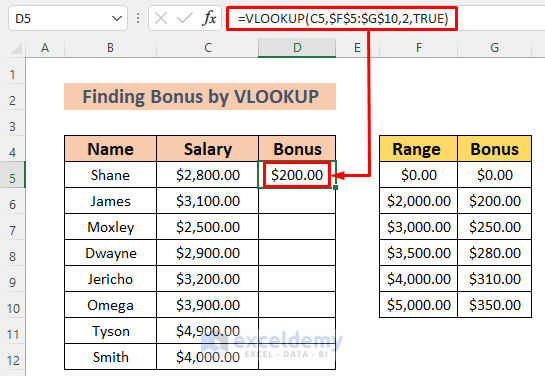
- Use the Fill Handle to AutoFill the Bonuses for the other Employees.
Example 2 – Find a Status Within a Time Range
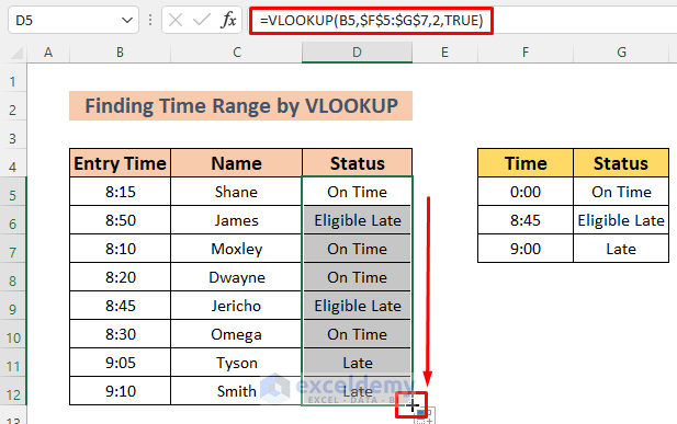
Let’s now use VLOOKUP to determine an Employee’s Status on a particular date (On Time, Eligible Late, or Late).
Steps:
- Again, we modify our dataset to contain appropriate data to demonstrate this method.
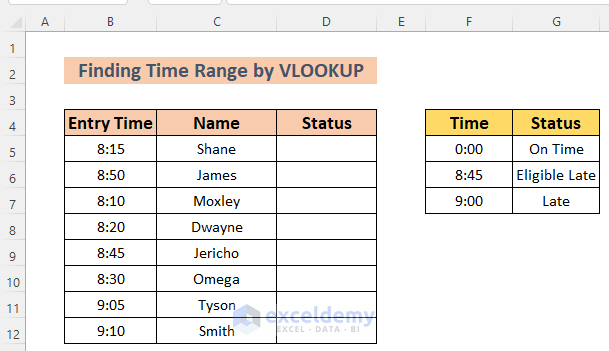
- Enter the following formula in cell D5:
=VLOOKUP(B5,$F$5:$G$7,2,TRUE)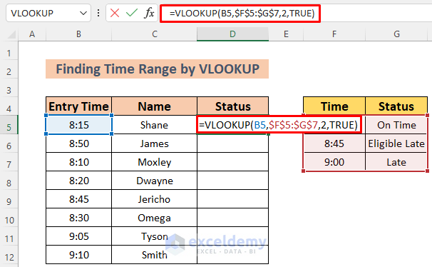
Here, the VLOOKUP Function looks for the Entry Time in cell B5 within the range F5:G7. As we want to determine the Status which is in the 2nd column of F5:G7, we set 2 as the col_index_num. We seek an approximate_match for the Entry Time in cell B5 within the Time range (F5:F7), so we set [range_lookup] as TRUE. We again use an absolute cell reference to enable accurate copying of this formula to calculate the Status of other Employees.
- Press ENTER to return the Entry Time Status of Shane.
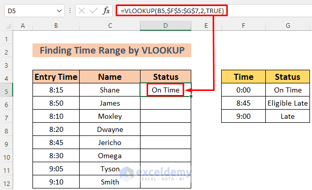
- Use the Fill Handle to AutoFill for the other Employees.
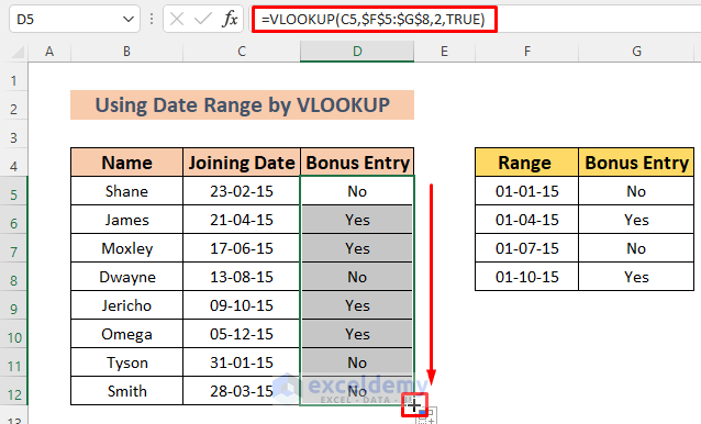
Example 3 – Find Bonus Entry Within a Date Range
VLOOKUP function can also be useful to find date values from a date range. Suppose only the employees who commence within a particular date range get Bonuses, while the rest don’t. For instance, only if Employees commenced between April and June are they due a bonus. Let’s determine who is due a Bonus.
Steps:
- Again, we modify our dataset with appropriate data to demonstrate this example.
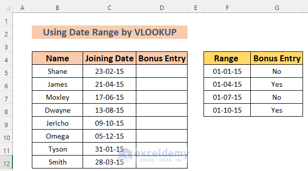
- Enter the following formula in cell D5:
=VLOOKUP(C5,$F$5:$G$8,2,TRUE)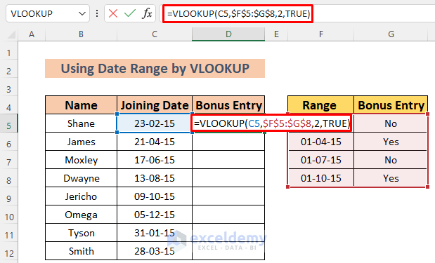
Here, the VLOOKUP Function looks for the Joining Date in cell C5 within the range F5:G8. As we want to determine the Bonus Entry which is in the 2nd column of F5:G8, we set 2 as col_index_num. We seek an approximate_match for the Joining Date in the Range range (cells F5:F8), so we set [range_lookup] as TRUE. We again use an absolute cell reference because the lookup range will remain the same for all Employees.
- Press ENTER to return the Bonus Entry Status of Shane.
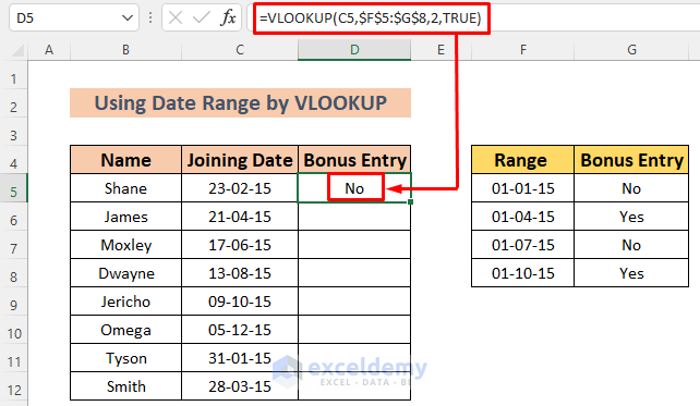
- Use the Fill Handle to AutoFill for the other Employees.
Example 4 – Using VLOOKUP with Combined Functions to Find a Value That Falls Within a Range
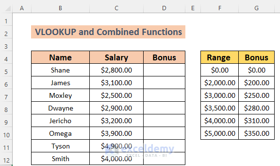
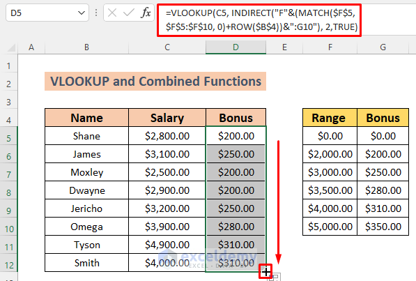
We can also determine the bonuses of these Employees by using the combination of VLOOKUP, INDIRECT, MATCH, and ROW Functions.
In the dataset, we set bonuses according to the salary range. For instance, those who have salaries in the range of $2000-2999 receive a bonus of $200; those who have salaries in the range of $3000-3499 receive a bonus of $250 and so on.
Steps:
- For this example, we return to the modified dataset we used in Example 1 above.
- Enter the following formula in cell D5:
=VLOOKUP(C5, INDIRECT("F"&(MATCH($F$5, $F$5:$F$10, 0)+ROW($B$4))&":G10"), 2,TRUE)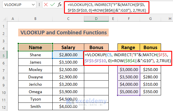
Formula Breakdown
Here, we use the INDIRECT, MATCH and ROW Functions to define the lookup range.
- ROW($B$4) —-> returns
- Output: {4}
- MATCH($F$5, $F$5:$F$10, 0) —->returns
- Output: 1
- MATCH($F$5, $F$5:$F$10, 0)+ROW($B$4) —->returns
- Output: {5}
- “F”&(MATCH($F$5, $F$5:$F$10, 0)+ROW($B$4))&”:G10″ —-> returns
- Output: F5:G10
- INDIRECT(“F”&(MATCH($F$5, $F$5:$F$10, 0)+ROW($B$4))&”:G10″) —-> becomes
- INDIRECT(F5:G10) —-> returns
- Output: the table_array for VLOOKUP (F5:G10)
- VLOOKUP(C5, INDIRECT(“F”&(MATCH($F$5, $F$5:$F$10, 0)+ROW($B$4))&”:G10″), 2,TRUE) —->returns
- Output: $200.00
The Bonus for Shane, $200, is returned.
- Press ENTER to return it.
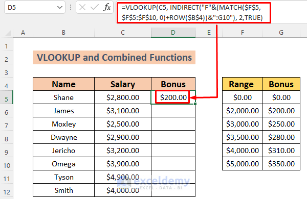
- Use the Fill Handle to AutoFill the Bonuses for the other Employees.
Example 5 – Using VLOOKUP and MATCH Functions to Find a Value That Falls Within a Range
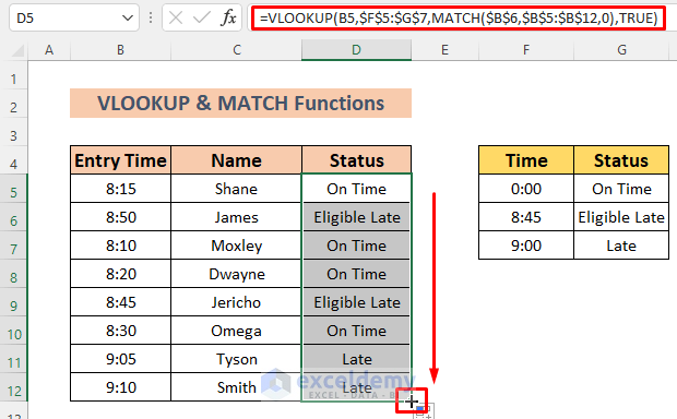
We can also use VLOOKUP combined with the MATCH function to accomplish the task in Example 2, ie to determine the Status (late or not) of the Employees on a day.
Steps:
- We use the same appropriately modified dataset as in Example 2 here again.
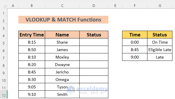
- Enter the following formula in cell D5:
=VLOOKUP(B5,$F$5:$G$7,MATCH($B$6,$B$5:$B$12,0),TRUE)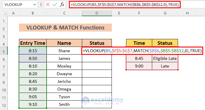
The VLOOKUP Function looks for the Entry Time in cell B5 within the range of F5:G7. As we want to determine the Status which is in the 2nd column of F5:G7, we set 2 as col_ index_num with the help of the MATCH function. We seek an approximate_match for the Entry Time in the Time range (cells F5:F7), so we set [Range Lookup] as TRUE. Again, to enable copying the formula to other Employees accurately, we use an absolute cell reference.
- Press ENTER to return the Entry Time Status of Shane.
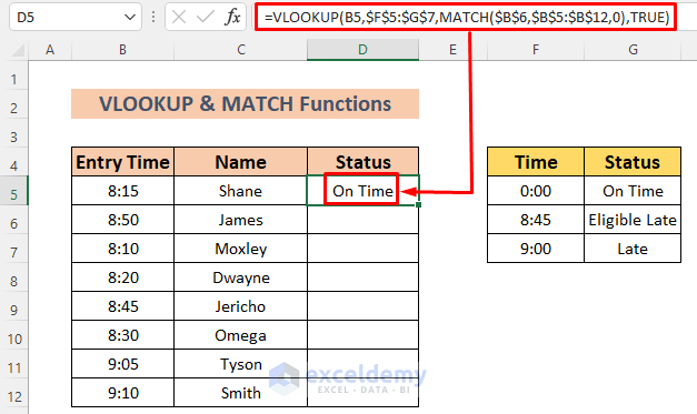
- Use the Fill Handle to AutoFill for the other Employees.
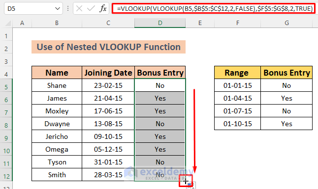
6. Applying Nested VLOOKUP to Find a Value That Falls Between a Range
Let’s now use nested VLOOKUP functions to re-do Example 3 above, namely to determine whether Employees are due a Bonus based on their commencement date.
Steps:
- We use the dataset modified for Example 3 here.
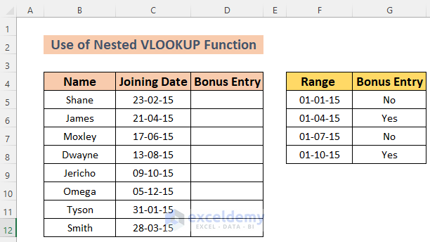
- Enter the following formula in cell D5:
=VLOOKUP(VLOOKUP(B5,$B$5:$C$12,2,FALSE),$F$5:$G$8,2,TRUE)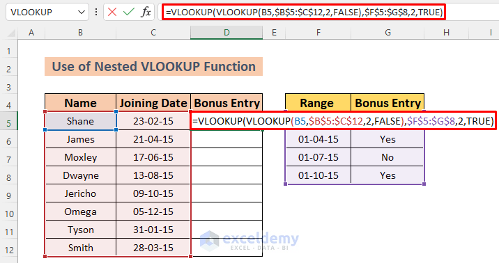
Here, the nested VLOOKUP Function returns the cell reference of C5, which refers to the Joining Date of C5. The main VLOOKUP Function then looks for cell reference C5 in the range of F5:G8. As we want to determine the Bonus Entry which is in the 2nd column of F5:G8, we set 2 as col_index_num. We seek an approximate_match for the Joining Date in the Range range (cells F5:F8), so we set [range_lookup] as TRUE. To enable accurate copying of the range reference F5:G8, we use an absolute cell reference.
- Press ENTER to return the Bonus Entry Status of Shane.
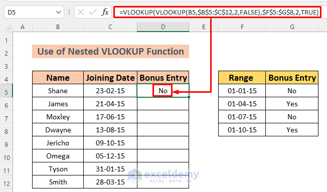
- Use the Fill Handle to AutoFill for the other Employees.
Things to Remember
When you set the range for Bonus or Entry Time or Date Range, the reference range must be sorted in ascending order. For example, in the case of setting Bonuses according to the Salary Range, $3000.00 should not appear before $2000.00 in the Range column.
Download Practice Workbook
Related Articles
- Vlookup with Time Range in Excel
- How to Use VLOOKUP If Condition Lies Between Multiple Ranges in Excel
<< Go Back to VLOOKUP a Range | Excel VLOOKUP Function | Excel Functions | Learn Excel
Get FREE Advanced Excel Exercises with Solutions!

