Example 1 – Count the Occurrences Using VLOOKUP and COUNTIF Functions
Let’s consider a dataset of student attendance over a week (based on student IDs) where we’ll calculate the total attendance of a student.
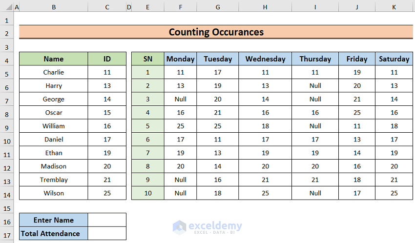
Steps:
- Select the C16 cell and type any name in the cell.
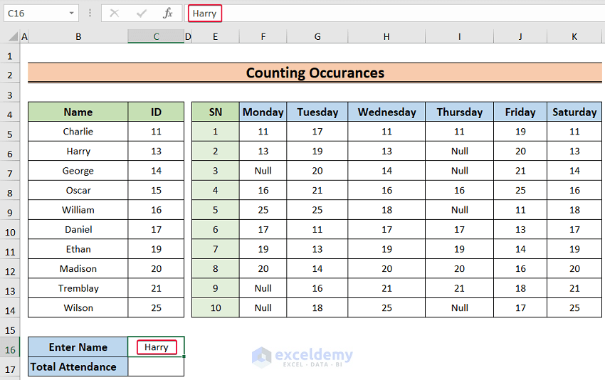
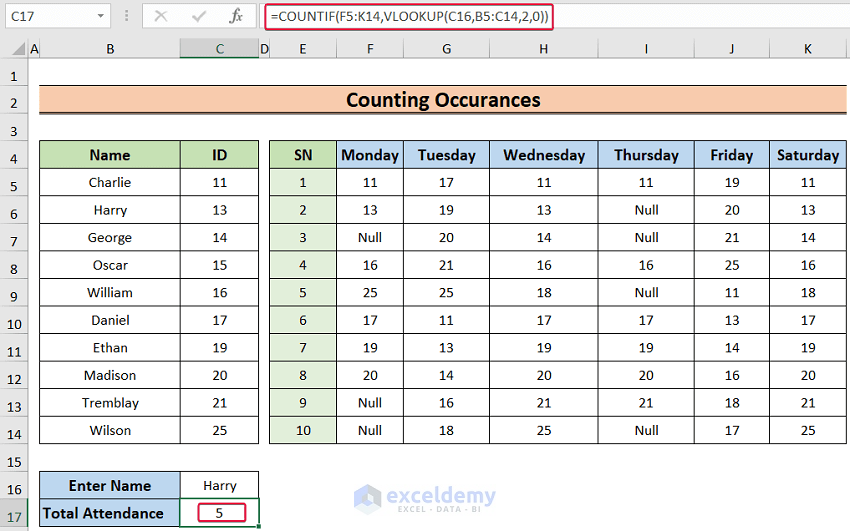
- Choose the C17 cell and insert the following:
=COUNTIF(F5:K14,VLOOKUP(C16,B5:C14,2,0))- Hit Enter.
Formula Breakdown:
- VLOOKUP(C16,B5:C14,2,0): The VLOOKUP function will match the value in the C16, lookup value, in the lookup range B5:C14. It returns the number associated with the name in the C16 cell in the second column of the range (student ID)
- COUNTIF(F5:K14,VLOOKUP(C16,B5:C14,2,0)): The COUNTIF function counts the number returned by the VLOOKUP(C16,B5:C14,2,0) expression (student ID) in the F5:K14 range and returns the number of appearances of that value.
Read More: How to Use IF ISNA Function with VLOOKUP in Excel
Example 2 – Calculate Percentages Using VLOOKUP and COUNTIF functions
We have a dataset of student marks for each course. We’ll find the average percentages of all the grades for a student if there are at least 4 grades. If a student has fewer than 4 recorded scores, we’ll simply return #NA!
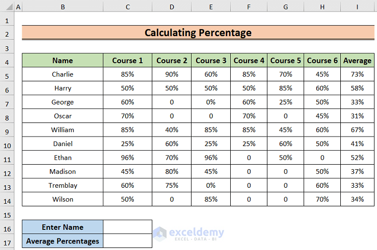
Steps:
- Choose the C16 cell and enter any name in the cell.
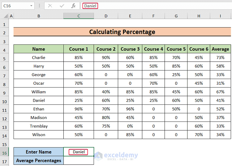
- Select the C17 cell and enter the following formula:
=IF(COUNTIF(INDEX($C$5:$H$14,MATCH(C16,$B$5:$B$14,0),0),">0")<4,NA(),VLOOKUP(C16,$B$5:$I$14,8,0))- Press Enter.
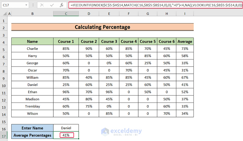
- VLOOKUP(C16,$B$5:$I$14,8,0): returns the [value_if_false] argument of the IF function. It is basically the average percentage of the obtained marks by the student.
- Output: 41%
- NA(): will return an error if the logical test argument of the IF function becomes TRUE. Here, Daniel attended more than 4 courses which is not the desired condition, so this part will return an error.
- Output: #N/A
- MATCH(C16,$B$5:$B$14,0): it will return the relative position of Daniel in the cell range B5:B14.
- Output: 6
- INDEX($C$5:$H$14,MATCH(C16,$B$5:$B$14,0),0) —-> simplifies to
- INDEX($C$5:$H$14,6),0): returns the set of percentages for Daniel.
- Output: {0.25,0.6,0.25,0.25,0.6,0.5}
- COUNTIF(INDEX($C$5:$H$14,MATCH(C16,$B$5:$B$14,0),0),”>0″) —-> turns into
- COUNTIF({0.25,0.6,0.25,0.25,0.6,0.5},”>0″): counts the percentages if the value is greater than 0.
- Output: 6
- The whole formula simplifies to IF(6<4, #N/A, 41%), which returns the average percentage of Daniel as 6<4 is not true.
- Output: 41%.
Read More: INDEX MATCH vs VLOOKUP Function
Example 3 – COUNTIF vs VLOOKUP for Determining If a Value Exists
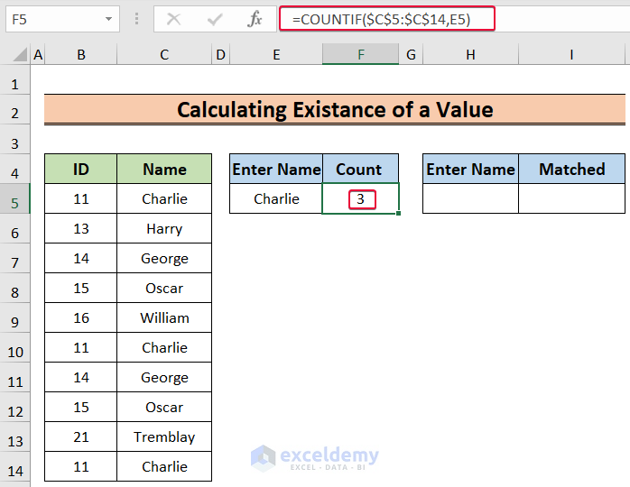
We have a dataset of employees with their names and IDs. There are repeated values in the table. We will count the names and try to match them.
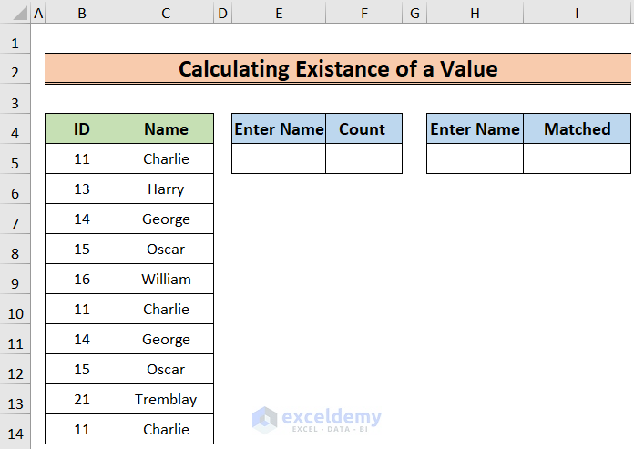
Steps:
- Click on the E5 cell and any name.
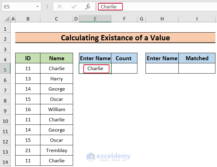
- Select the F5 cell and enter the following formula:
=COUNTIF($C$5:$C$14,E5)- Press Enter.
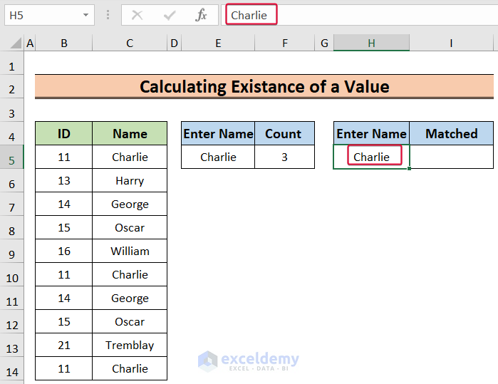
- Choose the H5 cell and any of the names.
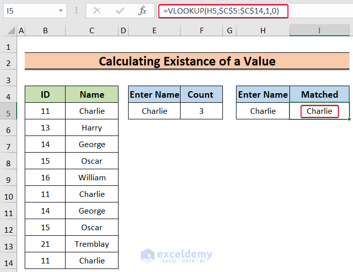
- Choose the I5 cell and enter the following:
=VLOOKUP(H5,$C$5:$C$14,1,0)- We will get the same name as in the H5 cell in the I5 cell.
Read More: Excel LOOKUP vs VLOOKUP
Download the Practice Workbook
Further Readings
- Combining SUMPRODUCT and VLOOKUP Functions in Excel
- How to Combine SUMIF and VLOOKUP in Excel
- Use VLOOKUP to Sum Multiple Rows in Excel
- XLOOKUP vs VLOOKUP in Excel
- How to Use Nested VLOOKUP in Excel
- IF and VLOOKUP Nested Function in Excel
- How to VLOOKUP and SUM Across Multiple Sheets in Excel
- How to Use IFERROR with VLOOKUP in Excel
- VLOOKUP with IF Condition in Excel
<< Go Back to Excel VLOOKUP Function | Excel Functions | Learn Excel
Get FREE Advanced Excel Exercises with Solutions!

