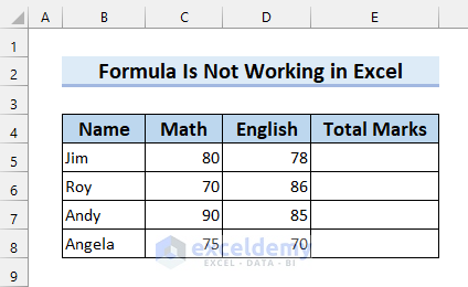
We’ll use a dataset that contains student Names and their scores in Math and English. We will go through some of the most common fixes when formulas fail to apply in Excel.
Fix 1 – Check Cell Format
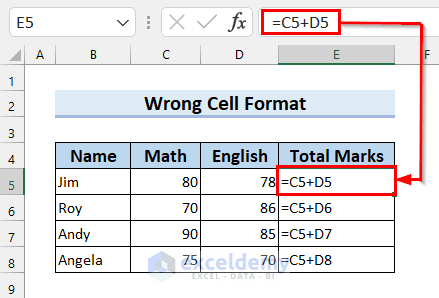
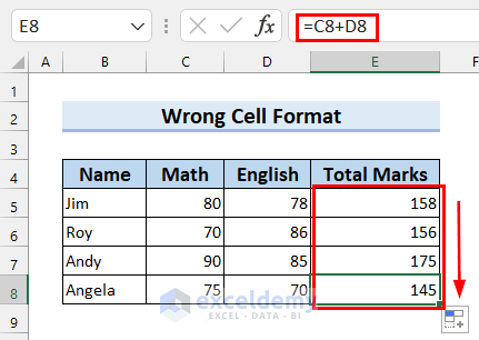
If you type the formula and see results like the picture shown below, you are seeing the formula as text. You have probably put the cell format as Text.
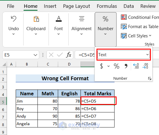
Go to the Number Format of the Home ribbon and check if Text is selected.
Solution:
- Select the cell that is showing this error. W selected cell E5.
- Go to Number Format on the Home ribbon and select General.
- Press Enter.
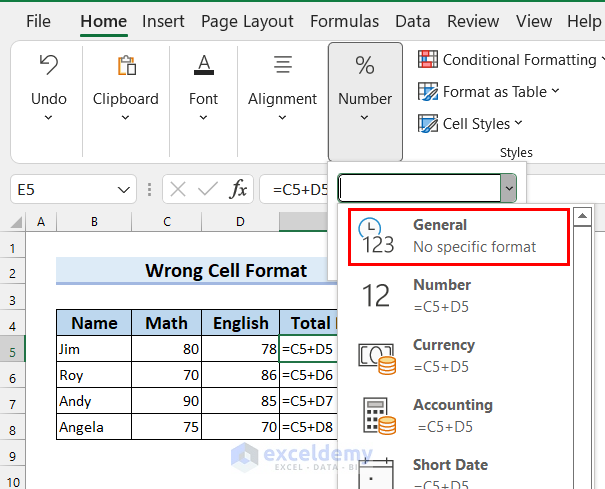
- Drag the Fill Handle and you will get your desired results in all the other cells.

- The formulas should start working.
Fix 2 – Check for a Space Before the Formula
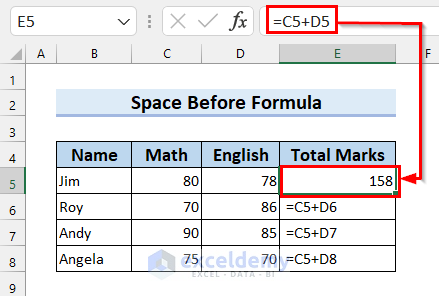
If the formulas still display as texts in the General format, there could be a space in front of the equals sign.
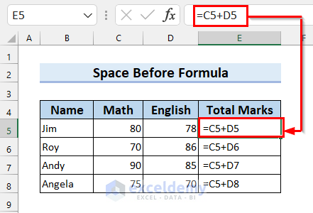
Select the cell where this problem is showing and check for a space before the formula.
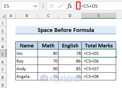
Solution:
- Select the cell where this problem is showing. We selected cell E5.
- Delete the space before the formula.
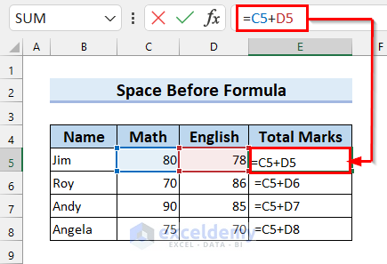
- Press Enter and you will get the correct result in that cell.
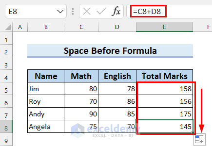
- Drag the Fill Handle to copy this formula to all the other cells.
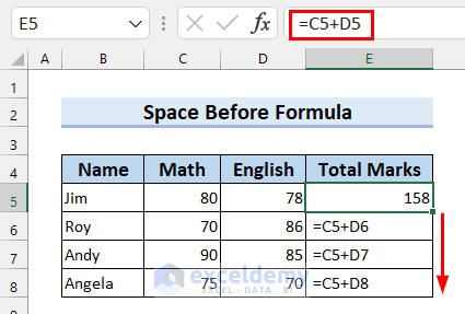
Alternatively, you can manually go through cells to correct them.
Fix 3 – Check If Formulas Are Enclosed in Double Quotes
If you put a formula in quotes, it will be used as a string value instead of a formula.
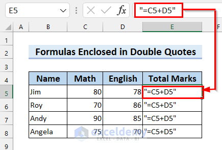
Solution:
- Delete the double quotes from the formula.
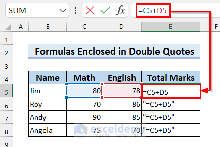
- Press Enter to apply the formula.
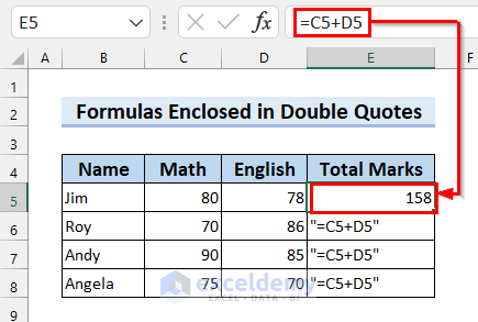
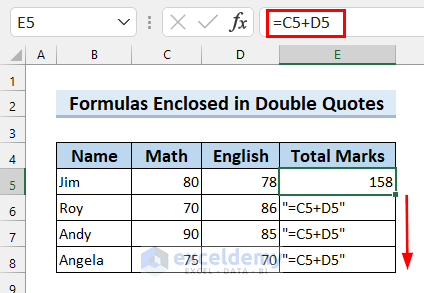
- Drag the Fill Handle to copy the formula to all the other cells if needed.
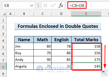
- We have the correct result for all the cells and the formula is working properly.
Fix 4 – Check If Numbers Are Enclosed in Double Quotes
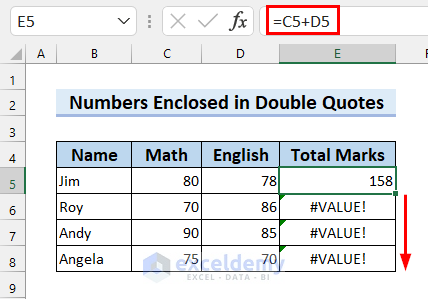
If a cell reference is in quotes, it won’t work in most formulas. The formula will return a #VALUE! error.
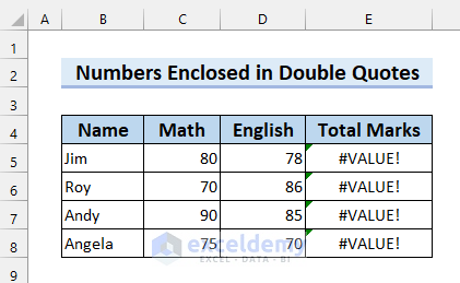
Select the cell and check the Formula Bar to see if this is the problem.
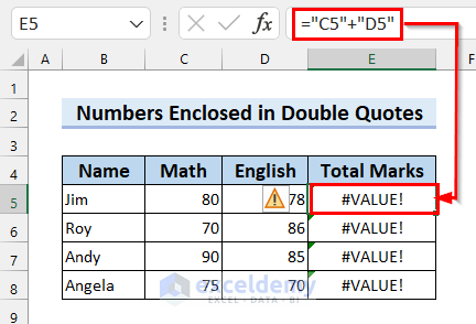
Solution:
- Select the cell where the error is showing.
- Remove the double quotes from the cell references.
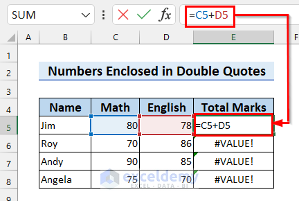
- Press Enter and you will get the correct result for the cell.
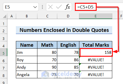
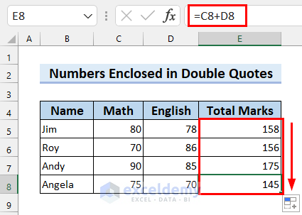
- Drag the Fill Handle to copy the formula to the rest of the cells.
- Here’s the result.
Read More: [Fixed]: Excel Formula Not Showing Correct Result
Fix 5 – Check for Circular References
If the formula fails to return a value, it could be trying to reference the cell it’s in for computation (a circular reference).
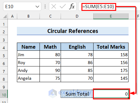
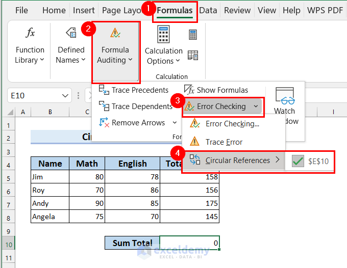
Here’s how you can check the Circular References.
- Go to the Formulas tab.
- Go to Formula Auditing.
- Click Error Checking.
- Put your cursor over Circular References. That will show you the cell that is causing this problem. Here, the cell E10 contains Circular References.
Solution:
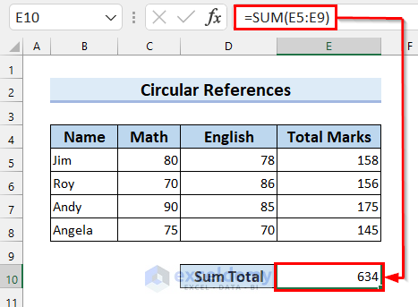
- Fix the range or cell references in the formula that is causing the Circular references. Here, E10 is causing the problem so we removed it from the formula.
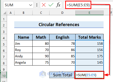
- Press Enter and you will see that your formula is working.
Fix 6 – Entering Numbers with Formatting
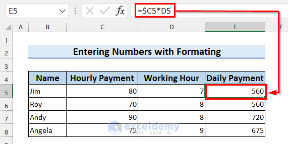
For this example, we want a currency ($) sign in the result but putting the currency sign in the formula doesn’t seem to work. This is because currencies are processed in a separate cell format. The $ sign is used to lock the row or column reference for the cell.
Solution:
- Select the cell where you want the currency ($) sign.
- Delete the currency ($) sign from the formula.
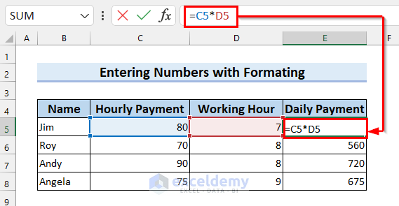
- Press Enter and you will get the result for the cell.
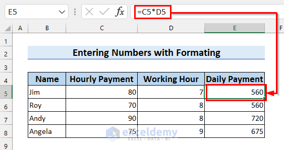
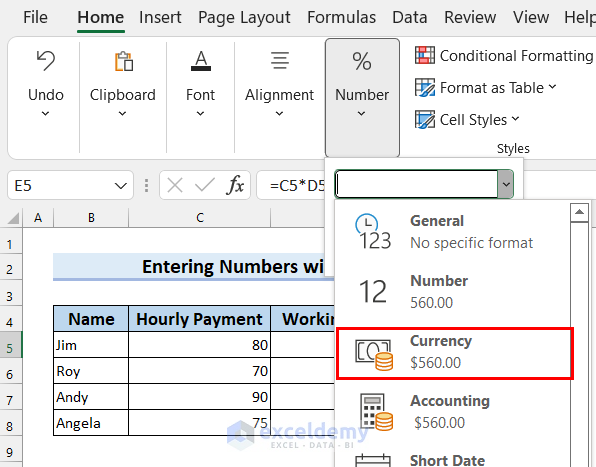
- Go to Number Format on the Home ribbon and select Currency.
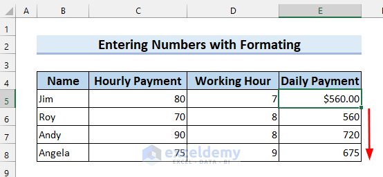
- You will get the currency ($) sign in your desired cell.
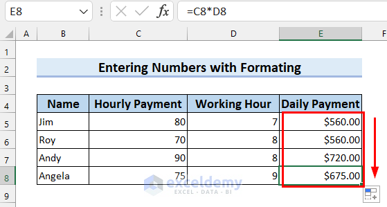
- Drag the Fill Handle to get the Currency formal in other cells.
- Here are the results.
- You can change the currency symbol by going to Format Cells.
Fix 7 – Check If the Automatic Calculation Option Is Selected
In this case, the first cell with the formula produces the correct result.
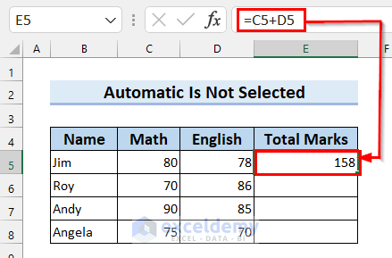
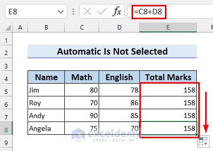
But, when you drag the Fill Handle to copy the formula to the other cells, the formula is not working as it’s supposed to.
One of the possible reasons behind this is that Manual Calculation is selected. With this option, Excel doesn’t calculate formula results until you force it to.
Solution:
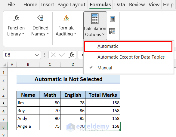
- Go to the Formulas tab.
- Go to the Calculations Option.
- Select Automatic.
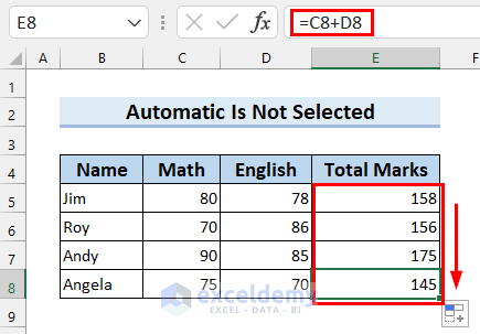
- You will see that your formula is working and you are getting the correct results.
Read More: [Fixed!] SUM Formula Not Working in Excel
Fix 8 – Check If You Have Deleted a Reference Row, Column, or Cell
If you see a #REF! error like the following image, you may have deleted a reference that the function used.
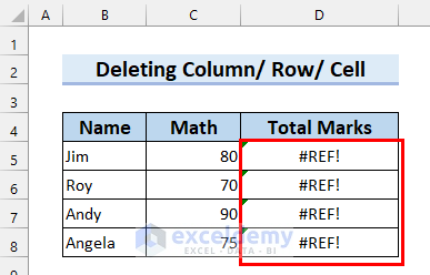
Select the cell that is showing the error. We selected cell D5.
Check the formula and see if there are any missing values.
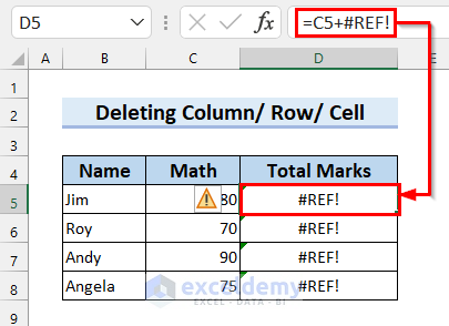
Solution:
- Unfortunately, you might not be able to undo cell deletion, so be careful when removing cells from the dataset.
- Readjust the formula.
Fix 9 – Check All Opening and Closing Parentheses
In the following image, we wanted to calculate the Total Percentage, but we are not getting the correct results. Since we didn’t use the parenthesis, the C5 value is being converted to 8000% for the calculation.
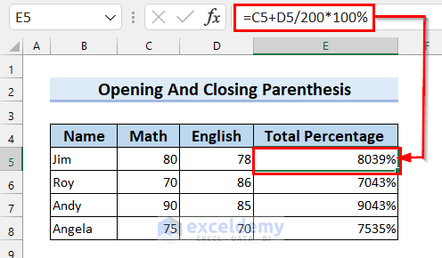
Solution:
- Select the cell where the problem is showing. We selected cell E5.
- Insert parentheses by following the PEMDAS or BODMAS rule to fix the formula.
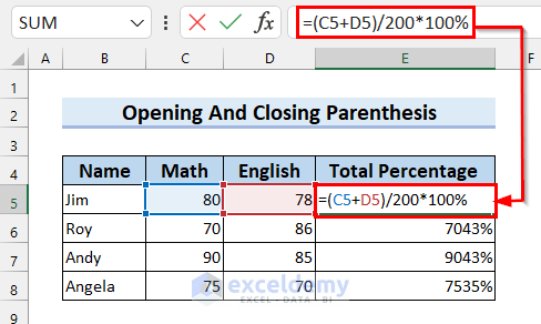
- Press Enter.
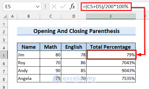
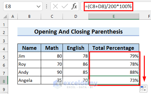
- Drag the Fill Handle to copy the formula to the rest of the cells.
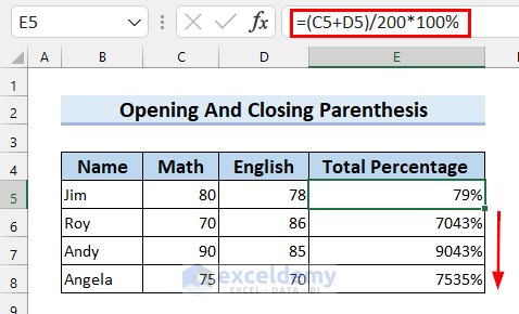
- You will see that your formula is working and you are getting all the correct results.
Fix 10 – Check If All Required Arguments Are Entered Properly
Consider the following dataset with the #N/A error.
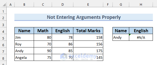
We used a VLOOKUP function and wrote the formula as shown below.
=VLOOKUP(G5,B5:E8,3)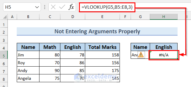
Here, I took G5 as lookup_value, B5:E8 as table_array, and 3 as col_index_number. But, I left the range_lookup blank. The formula isn’t working since the default value is TRUE for an approximate match, and this type of searching doesn’t work for unsorted string arrays.
Solution:
- Select the cell where the error is showing. Here, I selected cell H5.
- Write the formula correctly with all the arguments. We used the following formula.
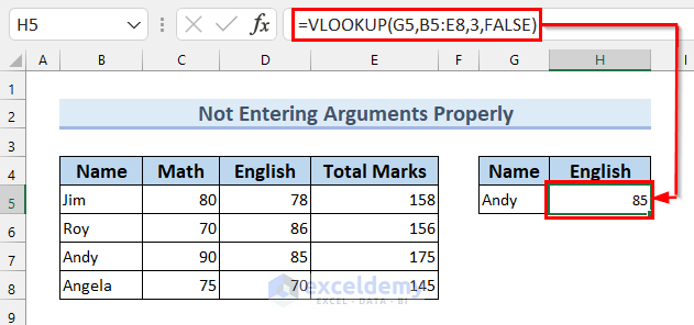
=VLOOKUP(G5,B5:E8,3,FALSE)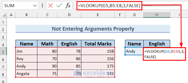
Here, I have selected G5 as lookup_value, B5:E8 as table_array, 3 as col_index_number, and FALSE as range_lookup. Now, I have entered all the arguments properly.
- Finally, press ENTER and you will see that the formula is working properly and giving you the correct answer.
 Read More: [Solved]: Excel Array Formula Not Showing Result
Fix 11 – Check for Incorrect Syntax of Function
A formula might not be working because the syntax is wrong for the use.
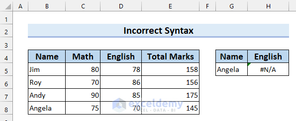
To check this, select the cell where the error is showing. We selected cell H5. Here’s the formula in the cell.
=VLOOKUP(G5,B5:E8,3,TRUE)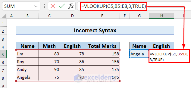
Here, I have selected G5 as lookup_value, B5:E8 as table_array, 3 as col_index_number, and TRUE as range_lookup. The problem with this formula is I selected TRUE as range_lookup while I want an exact match for the lookup_value.
TRUE is for approximate match and FALSE is for an exact match. While this might not matter, the problem is that “Jim” is considered to be “below” the string “Angela” if the array is sorted, and the function isn’t finding a value.
Solution:
- Select the cell where you want the correct result. We selected cell H5.
- Write the formula properly will all the correct syntax. We wrote the following formula.
=VLOOKUP(G5,B5:E8,3,FALSE)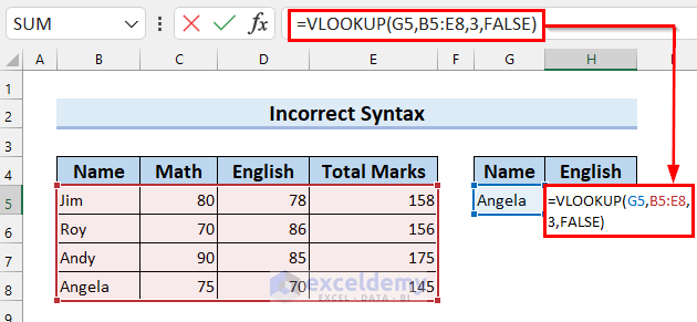
Here, we have selected G5 as lookup_value, B5:E8 as table_array, 3 as col_index_number, and FALSE as range_lookup. We have entered all the syntax correctly.
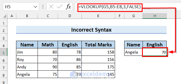
- Press Enter and you will see that the formula is working and giving you the correct result.
Fix 12. Check Whether Cell References Are Absolute or Relative
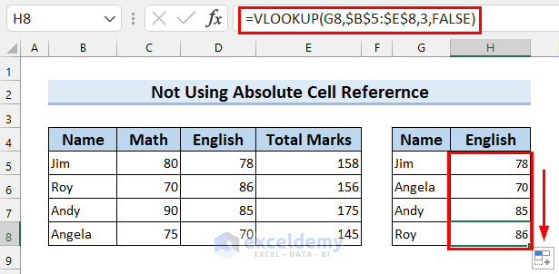
In the following example, some results are working and others are showing errors. This might be due to lack of absolute cell references in the formula.
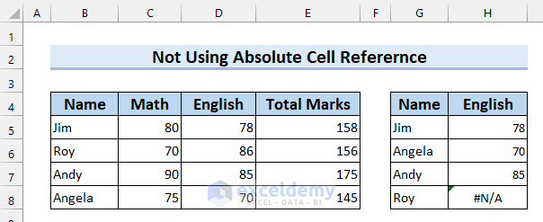
Select the formula cell and look at the formula bar to see the formula. We have selected cell H5, which contained the following.
=VLOOKUP(G5,B5:E8,3,FALSE)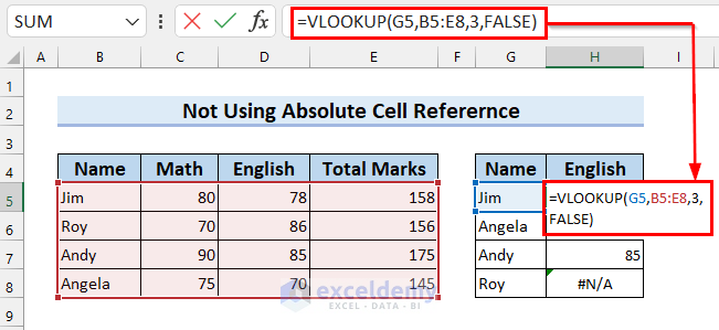
Here, I have selected G5 as lookup_value, B5:E8 as table_array, 3 as col_index_number, and FALSE as range_lookup. There is nothing wrong with this formula if you are writing this for that particular cell. But, when you drag the Fill Handle to copy the formula to the other cells, the cells in the formula will iterate accordingly. For the next cell, the table_array has moved one row down, which has started to effectively remove searchable values.
Solution:
- Select the first cell with the formula.
- Alter the formula to include absolute cell references for lookup arrays:
=VLOOKUP(G5,$B$5:$E$8,3,FALSE)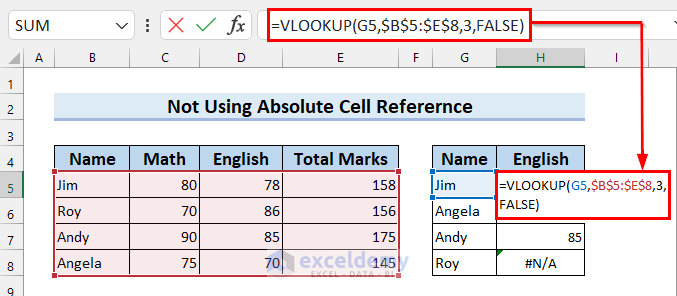
Here, I have selected G5 as lookup_value, B5:E8 as table_array, 3 as col_index_number, and FALSE as range_lookup. We used an absolute cell reference for the table_array so that the selected range remains fixed while using Autofill.
- Press Enter.
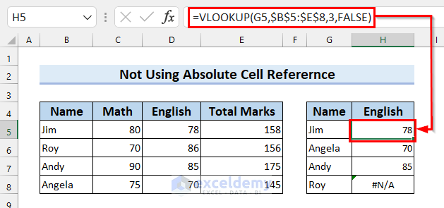
- Drag the Fill Handle to copy the new formula to all the other cells.
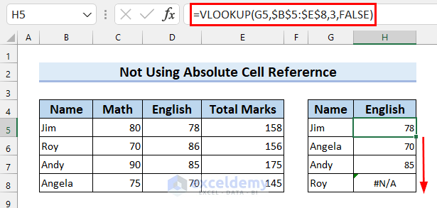
- The new formula works properly.
Fix 13 – Check If a Full Path to a Closed Workbook Is Included
Here’s an example of a formula that references another workbook, where we’re getting the #REF! error.
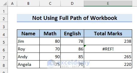
In cell E5, which contains the error, the formula is:
=C5+D5+'[Biology.xlsx]Biology'!C5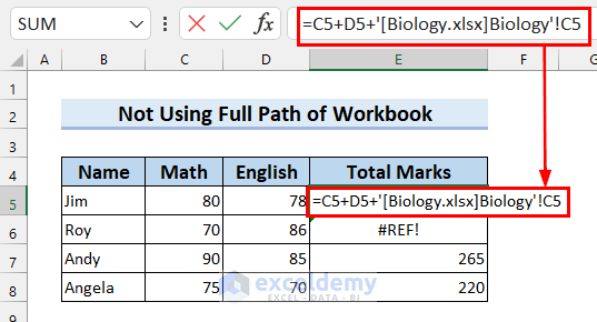
We summed cells C5 and D5, as well as cell C5 from another workbook named Biology.xlsx and the worksheet named Biology. The problem with this formula that the worksheet is closed, and Excel can’t find the value without a full file path.
Solution:
- Select the cell with an error.
- Insert the full file path before the workbook name like the following. You will need to find your workbook’s file path manually.
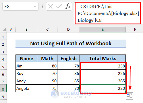
=C5+D5+'E:\This PC\Documents\[Biology.xlsx]Biology'!C5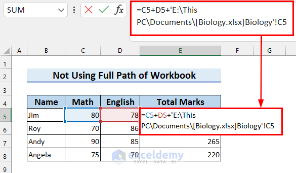
- Press Enter and you will get the correct result.
- Drag the Fill Handle to copy the formula to all the other cells if needed.
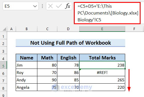
- The formula is working properly.
Fix 14 – Enclosing Workbook or Worksheet in Double Quotes
If you accidentally or intentionally enclose the worksheet name in a double quote in the formula, then the formula will show an error like the image below.
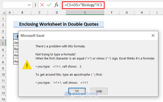
Solution:
- Select OK to close the error message.
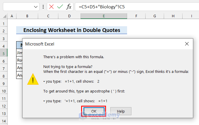
- Select the cell where the error is showing.
- Remove the quotes from sheet names.
=C5+D5+Biology!C5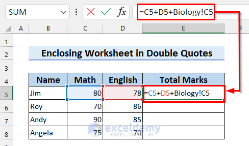
- Press Enter.
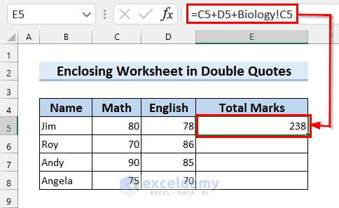
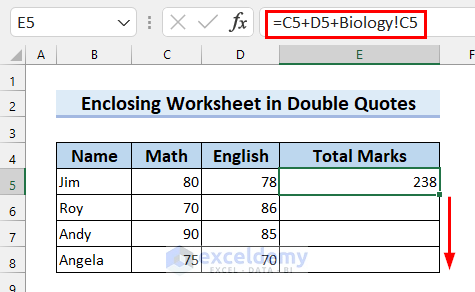
- Drag the Fill Handle to copy the formula to all the other cells.
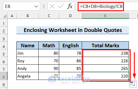
- Here are the results.
Fix 15 – Nesting More than the Allowed Number of Functions
Solution:
- If you are using Excel 2003 or lower, you can use up to 7 nested functions.
- If you are using Excel 2007 or newer, you can nest up to 64 nested functions.
Download the Practice Workbook
Knowledge Hub
- How to Refresh Formulas in Excel
- [Fixed!] Formula Not Working and Showing as Text in Excel
- Excel Formulas Not Calculating Automatically
- [Fixed!] Excel Formulas Not Working on Another Computer
- [Solved:] Excel Formula Not Working unless Double Click Cell
- [Solved]: Excel Formulas Not Updating Until Save
<< Go Back To Excel Formulas | Learn Excel
Get FREE Advanced Excel Exercises with Solutions!

