| STUDENT NAME | Annual Fee | Discount | Final Fee | Book Amt | Date | 1st Pay | Date | 2nd Pay | Date | 1st Instal Amt | 1st Instal Bal |
| Aaroh | 24000 | 720 | 23280 | 2000 | 15-02-23 | 21280 | 03-04-23 | 0 | | 0 | 0 |
| Vedika | 26800 | 1434 | 25366 | 2000 | 20-02-23 | 5500 | 03-05-23 | 0 | | 8455 | 955 |
| Anvee | 22500 | | 22500 | 2000 | 17-02-23 | 7500 | 27-04-23 | 0 | | 7500 | -2000 |
| Jiggisha | 22500 | | 22500 | 2000 | 21-02-23 | 5500 | 04-05-23 | 0 | | 7500 | 0 |
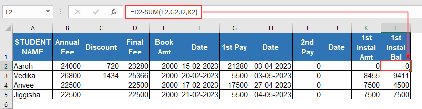
In the Last column, Instal Bal
I want to avoid -ve numbers.
Presently I'm using the sum formula as such that it shows +ve numbers only if the instalment amount is pending ( receivable)
thus making excess amount showing in -ve.
How can I avoid such -ve amount
and have the excess amount being added in the next instalment balance adjusted,
Hello
Nikhil Patki,
Thanks for reaching us. I understand that you want to avoid -ve numbers in the
1st Instal Bal column. You also want the excess amount to be added to the next installment balance when adjusted.
We can accomplish your requirements using two simple formulas using
MAX,
MIN, and
ABS functions. However, I am unclear about the formula you have used to calculate the 1st Instal Bal column values.
To get the actual solution to your problem, please share a sample Excel workbook or the formulas you used in your calculations. Otherwise, adjust your used formulas according to the following generic formulas:
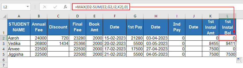
- For avoiding -ve in the 1st Instal Bal column, you can use-
=MAX(YourPreviousFormula,0)
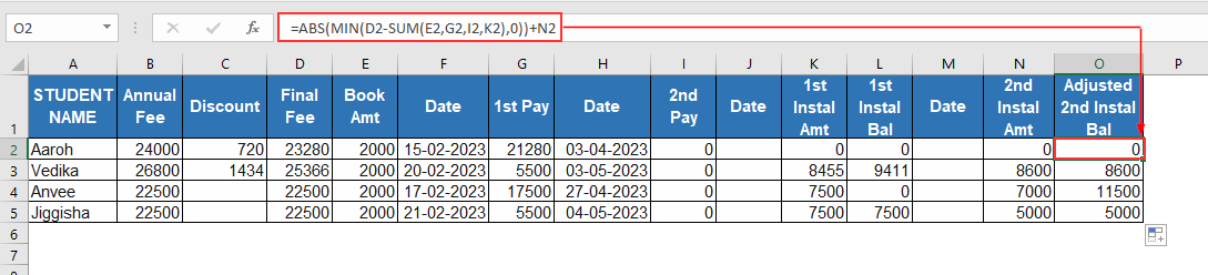
- To adjust the excess amount to the next installment balance, apply the following formula-
=ABS(MIN(YourPreviousFormula,0))+NextInstallmentValue
For instance, if you used
=D2-SUM(E2,G2,I2,K2) to calculate the
1st Instal Bal value.
To avoid -ve values here, you have to modify the formula to the following:
=MAX(D2-SUM(E2,G2,I2,K2),0)
And if you enter the next installment value (i.e. 2nd Instal Amt) in column
N and want the adjusted value in column
O, then you have to insert the following formula:
=ABS(MIN(D2-SUM(E2,G2,I2,K2),0))+N2
Hopefully, the above-demonstrated formulas will help you to find a solution to your problem. Let us know your feedback.
Regards,
Seemanto Saha
ExcelDemy