Index-Match Date format & Skipping Blank Cells

[yunus786]

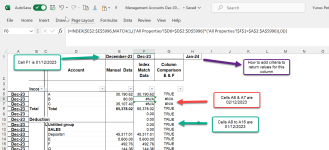
Below is a screenshot of my attempt of using Index Match formula for multiple criteria in Column F. Column E is my expected output.
I have 3 Questions for support on...
1) How do I fix the Index Match formulae for Cells F6 & F7. It does not return a value because the lookup Cells A6 & A7 respectively are 02/12/23 whereas the for the other cells it is 01/12/2023. I would like the lookup to be dynamic so it only looks up the month only not the day as well. This should then allow me to add a columns for other month i.e. Jan-2024 as in Column H and still execute the same formulae?

2) How to tell Index Match to skip blank values and keep on searching until it finds a non-empty value. I don't want the formulae to return any value should the array not have a value.. Presently it is returning 0.00.
3) Following on form point 2, the formulae goes pear shaped if the "Total" is only in cell B8 not D8. I had to move it to D8 to make it work correctly otherwise all blank cells in column D was returning value fron Cell F8. I accept in this method of using Index Match using Boolean. Is there another way of using Index Match to look up value regardless of the column it is in?

 

[MD Tanvir Rahman]

Below is a screenshot of my attempt of using Index Match formula for multiple criteria in Column F. Column E is my expected output.
I have 3 Questions for support on...
1) How do I fix the Index Match formulae for Cells F6 & F7. It does not return a value because the lookup Cells A6 & A7 respectively are 02/12/23 whereas the for the other cells it is 01/12/2023. I would like the lookup to be dynamic so it only looks up the month only not the day as well. This should then allow me to add a columns for other month i.e. Jan-2024 as in Column H and still execute the same formulae?

2) How to tell Index Match to skip blank values and keep on searching until it finds a non-empty value. I don't want the formulae to return any value should the array not have a value.. Presently it is returning 0.00.
3) Following on form point 2, the formulae goes pear shaped if the "Total" is only in cell B8 not D8. I had to move it to D8 to make it work correctly otherwise all blank cells in column D was returning value fron Cell F8. I accept in this method of using Index Match using Boolean. Is there another way of using Index Match to look up value regardless of the column it is in?

View attachment 1218

Dear [B]yunus786[/B], first of all, thank you so much for your query. Can you please send me the Excel file? So that it would be helpful for me to serve you with the appropriate answer.
Your problem is unique, so the answer should be creative too.
Have a good day.

Regards,
MD Tanvir Rahman
Excel and VBA Content Developer, ExcelDemy

 

[yunus786]

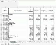
Here you go Tanvir. Using the data in Worksheet 'Attendance' I wish to populate the other tables, using Index/Match formulae. The Table is dynamic, monthly a new set of data is added.

 

[yunus786]

MD Tanvir Rahman
File attached

 

[MD Tanvir Rahman]

Below is a screenshot of my attempt of using Index Match formula for multiple criteria in Column F. Column E is my expected output.
I have 3 Questions for support on...
1) How do I fix the Index Match formulae for Cells F6 & F7. It does not return a value because the lookup Cells A6 & A7 respectively are 02/12/23 whereas the for the other cells it is 01/12/2023. I would like the lookup to be dynamic so it only looks up the month only not the day as well. This should then allow me to add a columns for other month i.e. Jan-2024 as in Column H and still execute the same formulae?

2) How to tell Index Match to skip blank values and keep on searching until it finds a non-empty value. I don't want the formulae to return any value should the array not have a value.. Presently it is returning 0.00.
3) Following on form point 2, the formulae goes pear shaped if the "Total" is only in cell B8 not D8. I had to move it to D8 to make it work correctly otherwise all blank cells in column D was returning value fron Cell F8. I accept in this method of using Index Match using Boolean. Is there another way of using Index Match to look up value regardless of the column it is in?

View attachment 1218

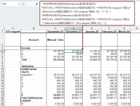
Dear @yunus786, thanks a ton for sending me the Excel file. I have used the INDEX-MATCH formula to call values from another sheet named Attendance. Here's how:
1. Use the following formula:
=IFERROR(INDEX(Attendance!$C$3:$C$273, MATCH(1, (MONTH(Attendance!$A$3:$A$273) = MONTH('All Leagues'!D$1))*(Attendance!$B$3:$B$273 = 'All Leagues'!$B4), 0)), "")
2. Use the Fill Handle to copy the formula.



The formula is not dynamic but it updates automatically if the value changes. To update automatically you can use VBA Macro where you will be able to add new data and call data automatically.

How Formula Works?
1. We converted the date into month first to match the month. So, we used the MONTH function that returns an integer value.
2. Then we matched the values of "column B" and the month using the MATCH function and AND operator.
3. To pull data we have used the INDEX function.
4. To eliminate any kind of error we applied the IFERROR function.

How to Avoid Blank Cells:
To avoid blank cells, you can apply the IF function with the IF-MATCH formula.
=IF(IFERROR(INDEX(Attendance!$C$3:$C$273, MATCH(1, (MONTH(Attendance!$A$3:$A$273) = MONTH('All Leagues'!D$1)) * (Attendance!$B$3:$B$273 = 'All Leagues'!$B4), 0)), "") = 0, "", IFERROR(INDEX(Attendance!$C$3:$C$273, MATCH(1, (MONTH(Attendance!$A$3:$A$273) = MONTH('All Leagues'!D$1)) * (Attendance!$B$3:$B$273 = 'All Leagues'!$B4), 0)), ""))



I have attached the Excel file. Please check out the formulas. For any other further shortcomings, please feel free to let us know. Have a good day.

Regards,
MD Tanvir Rahman
Excel and VBA Content Developer, ExcelDemy

 

[yunus786]

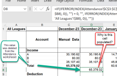
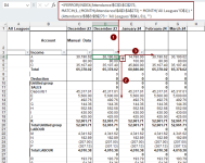
Thank you. This is great, but there is an anomaly....
1. If you delete the contents of any data from the Worksheet from where the data is pulled from e.g. Cell 'Attendance'B6 "Total", the formula, not only returns a blank or #N/A, as expected but it also populates the next cell down it populates the value which would have been in the previous cell above (see screenshot below) , that's wrong but why?
2. Did you apply the formatting manually in the "All Leagues" worksheet to match the attendance worksheet, as 'Fill Handle' does not apply formatting?
3. Thank you for the "Month" explanation", that's what I originally failed to understand

 

[MD Tanvir Rahman]

Thank you. This is great, but there is an anomaly....
1. If you delete the contents of any data from the Worksheet from where the data is pulled from e.g. Cell 'Attendance'B6 "Total", the formula, not only returns a blank or #N/A, as expected but it also populates the next cell down it populates the value which would have been in the previous cell above (see screenshot below) , that's wrong but why?
2. Did you apply the formatting manually in the "All Leagues" worksheet to match the attendance worksheet, as 'Fill Handle' does not apply formatting?
3. Thank you for the "Month" explanation", that's what I originally failed to understand

View attachment 1236

Dear @yunus786, please navigate the GIF below, it's working accurately. I see no anomaly. And Yes, you must format manually since the Fill Handle tool doesn't format automatically.



However, Excel sometimes tends to mess up. It's quite irritating. There are several reasons for not showing correct results in Excel:

1. Incorrect Formula: Double-check the formula for errors, typos, or incorrect references.
2. Cell References: Ensure that cell references in the formula are accurate and include the correct range.
3. Data Types: Check if data types are consistent; mixing text and numbers in calculations may lead to errors.
4. Cell Formatting: Verify that the cells involved in the calculation have the appropriate formatting, as formatting can affect the outcome.
5. Circular References: Avoid circular references where a cell refers to itself or creates a loop.
6. Hidden Characters: Look out for hidden characters or leading/trailing spaces in cell contents that may interfere with calculations.
7. Calculation Mode: Ensure Excel is set to automatic calculation mode, as manual mode may cause delays in updating formulas.
8. Error Values: Check for error values like #DIV/0! or #VALUE! that indicate problems in the formula.
9. Function Arguments: Make sure to provide the correct arguments and follow the syntax for functions used in the formula.
10. Data Accuracy: Confirm the accuracy of the data being used in calculations; errors in input data can lead to incorrect results.
11. Version Compatibility: Ensure that the Excel version you are using supports the functions and features used in the formula.

You can check out the below two articles to solve this issue.

• Why Formula Is Not Working in Excel
• Why Excel Formula Not Showing Correct Result

For any other further shortcomings, please feel free to let us know. Have a good day.

Regards,
MD Tanvir Rahman
Excel and VBA Content Developer, ExcelDemy