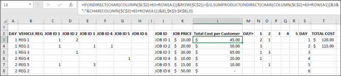
Please see below a simplified example of the spreadsheet I'm working on. This data will be on three separate tabs and I've got to keep the data in that format which is proving difficult with it effectively transposed.
I need to to calculate the total cost based on the day number, using the sum of each job id per day multiplied by their price rate. There will be a further variable as there will also be an individual column per customer on Revenue spreadsheet for total cost with individual tabs per customer but trying to master this before adding further variable. I've tried various combinations of SUMPRODUCT, IFS,SUMIFS, INDEX MATCH ETC (some examples in screenshot) but am either getting a returned #VALUE!, #N/A or total of all prices*the day number. (on the actual spreadsheet, the tab names! are inc. in the formula). Is this possible or am I just expecting too much?

I've managed to sum the number of jobs matching each job ID and day number. but can't extend this to calculate the total cost.
EDITED: =IF(M$2=$T3,SUMPRODUCT($M$3:M8,$K$3:$K$8),0), *RETURNS THE SUM * PRICE FOR EACH ROW, BUT NEED IT DYNAMICALLY TO INCLUDE ALL COLUMNS AS FORMULA NEEDS DRAGGING DOWN FOR 31 DAYS AND EVENTUALLY ACROSS MULTIPLE COLUMNS ONCE HAVE INDIVIDUAL CUSTOMER COLUMNS. I CAN ALSO GET IT TO SUM * PRICE USING (IF(AND() WHEN HAVE THE CUSTOMER TOTAL COST HEADER AND CUSTOMER NAME ON SERVICES TAB. CANNOT GET IT TO WORK WITHOUT SPECIFYING SPECIFIC COLUMNS AND MANUALLY AMENDING EACH TIME AND ONCE IT BECOMES POTENTIALLY 150 CELLS, WILL NEED A MORE EFFICIENT FORMULA#
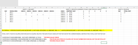
I need to to calculate the total cost based on the day number, using the sum of each job id per day multiplied by their price rate. There will be a further variable as there will also be an individual column per customer on Revenue spreadsheet for total cost with individual tabs per customer but trying to master this before adding further variable. I've tried various combinations of SUMPRODUCT, IFS,SUMIFS, INDEX MATCH ETC (some examples in screenshot) but am either getting a returned #VALUE!, #N/A or total of all prices*the day number. (on the actual spreadsheet, the tab names! are inc. in the formula). Is this possible or am I just expecting too much?
I've managed to sum the number of jobs matching each job ID and day number. but can't extend this to calculate the total cost.
EDITED: =IF(M$2=$T3,SUMPRODUCT($M$3:M8,$K$3:$K$8),0), *RETURNS THE SUM * PRICE FOR EACH ROW, BUT NEED IT DYNAMICALLY TO INCLUDE ALL COLUMNS AS FORMULA NEEDS DRAGGING DOWN FOR 31 DAYS AND EVENTUALLY ACROSS MULTIPLE COLUMNS ONCE HAVE INDIVIDUAL CUSTOMER COLUMNS. I CAN ALSO GET IT TO SUM * PRICE USING (IF(AND() WHEN HAVE THE CUSTOMER TOTAL COST HEADER AND CUSTOMER NAME ON SERVICES TAB. CANNOT GET IT TO WORK WITHOUT SPECIFYING SPECIFIC COLUMNS AND MANUALLY AMENDING EACH TIME AND ONCE IT BECOMES POTENTIALLY 150 CELLS, WILL NEED A MORE EFFICIENT FORMULA#
Attachments
Last edited: