How to put daily MLB Baseball Games results in Excel using VBA Code?

Boy282828 · Mar 31, 2024

Dear Sir,

In Excel 365 I have a consecutive (No Blank Cells) Column Array Selected in

some portion of Column C (Not beginning on C1) for example such as:

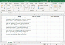
Colorado Rockies (1) @ Arizona D'Backs (16) Boxscore

Los Angeles Angels (3) @ Baltimore Orioles (11) Boxscore

Detroit Tigers (1) @ Chicago White Sox (0) Boxscore

Washington Nationals (2) @ Cincinnati Reds (8) Boxscore

New York Yankees (5) @ Houston Astros (4) Boxscore

Minnesota Twins (4) @ Kansas City Royals (1) Boxscore

St. Louis Cardinals (1) @ Los Angeles Dodgers (7) Boxscore

Pittsburgh Pirates (6) @ Miami Marlins (5) Boxscore

Cleveland Guardians (8) @ Oakland Athletics (0) Boxscore

San Francisco Giants (4) @ San Diego Padres (6) Boxscore

Boston Red Sox (6) @ Seattle Mariners (4) Boxscore

Toronto Blue Jays (8) @ Tampa Bay Rays (2) Boxscore

Chicago Cubs (3) @ Texas Rangers (4) Boxscore

I would like to have the VBA Code to run this Array all in once with

these results:

All the Visitor Baseball Teams WITHOUT the bracket Score Stay in Column C and Convert Team Names to 3 Letters Symbol according
to a Table Called “TMSYMBOL”, on that Table the 1st Column is all Team

Names, the 2nd Column is all Team Symbols, I use the Formula of

“=VLOOKUP( Selected Team Name , TMSYMBOL, 2 )” to convert

Team Names to 3 Letter Symbols manually for each Team Name but

waste lots of time. I want to select the whole Array of Column C so

it will show All Team 3 Letter Symbols right away.

To get rid of the Scores bracket I use the Built in Function

“=LEFT(Select Team, LEN(Select Team)-5)”, I did this 1st before

Using VLOOKUP Functions.

(2) To the right of each Team Name is the Score of that Team, e.g.

Colorado Rockies (1), which means Colorado Rockies Score is 1,

I would like to have all Team Scores extracted from that Team

and show them all in real Integer Numbers without any bracket()

to avoid Misleading for Excel to think it is a Negative Number.

The Integer Column Array is on Column D which is to the right side

of Column C Team Name Symbols with the same Row Numbers as

Column C.

(3) After all the “@” are the Home Team Names, their Scores in bracket,

and extra Tails of “Boxscore”, I use function “=LEFT(Selected team

name, LEN(Selected team name)-12) to get rid of the “Boxscore” Tails.

However there is a Catch for the Home Team Name Conversion to

3 Letter Symbol of Teams. Since After “@” there is a SPACE of each

Home Teams, I have to manually delete each First SPACE before the

Home Team Names, then I can do the VLOOKUP Convert to Symbols,

Could you write code so that it will delete ALL 1st space before each

Home Team Name, then Convert to 3 Letter Symbol Array on

Column H, extract the Home team scores on Column I with

the same Row Numbers, in other words, Parallel moving all

the Column Arrays. Eliminate al the “@” Symbol.

The Results are like these:

Column C Column D Column H Column I

AWAY TM V-SCORE HOME TM H-SCORE

COL	1	ARI	16
LAA	3	BAL	11
DET	1	CHW	0
WAS	2	CIN	8
NYY	5	HOU	4
MIN	4	KC	1
STL	1	LAD	7
PIT	6	MIA	5
CLE	8	OAK	0
SF	4	SD	6
BOS	6	SF	4
TOR	8	TB	2
CHC	3	TEX	4

It should be all in line, I just can’t do it in Words. Sorry about that.

In Excel they should have the same Row Numbers.

The Conversion Table named “TMSYMBOL” in my Excel Worksheet

named “TMS” is as follows

Arizona D'Backs	ARI
Atlanta Braves	ATL
Baltimore Orioles	BAL
Boston Red Sox	BOS
Chicago Cubs	CHC
Chicago White Sox	CHW
Cincinnati Reds	CIN
Cleveland Guardians	CLE
Colorado Rockies	COL
Detroit Tigers	DET
Houston Astros	HOU
Kansas City Royals	KC
Los Angeles Angels	LAA
Los Angeles Dodgers	LAD
Miami Marlins	MIA
Milwaukee Brewers	MIL
Minnesota Twins	MIN
New York Mets	NYM
New York Yankees	NYY
Oakland Athletics	OAK
Philadelphia Phillies	PHI
Pittsburgh Pirates	PIT
San Diego Padres	SD
Seattle Mariners	SEA
San Francisco Giants	SF
St. Louis Cardinals	STL
Tampa Bay Rays	TB
Texas Rangers	TEX
Toronto Blue Jays	TOR
Washington Nationals	WAS

( Each Team in ONE line only. )

The name of the worksheet is “SKD DOG”, the name of the Workbook is

“2024MLB”, due to everyday I have new data in Column C to update,

Could you modify the Code dynamically so that once I select today’s

Input Array in Column C ( It varies since today it starts with C10, but

tomorrow I have to start with C14 to get day by day schedule & score result).

The Heading of the Visitor Team name is “AWAY TM” on C6, the Heading of the

Visitor Score is “V-Score” on D6, the Heading of the Home Team Name is

“HOME TM” on H6, the Heading of the Home Team Score is “H-Score” on I6.

I hope I explained my expected results using VBA Code to run clearly.

If you need more information, please feel free to ask. Thanks.

Boy282828 3/30/2024

Lutfor Rahman Shimanto · Mar 31, 2024

Boy282828 said:
Dear Sir,

In Excel 365 I have a consecutive (No Blank Cells) Column Array Selected in

some portion of Column C (Not beginning on C1) for example such as:

Colorado Rockies (1) @ Arizona D'Backs (16) Boxscore

Los Angeles Angels (3) @ Baltimore Orioles (11) Boxscore

Detroit Tigers (1) @ Chicago White Sox (0) Boxscore

Washington Nationals (2) @ Cincinnati Reds (8) Boxscore

New York Yankees (5) @ Houston Astros (4) Boxscore

Minnesota Twins (4) @ Kansas City Royals (1) Boxscore

St. Louis Cardinals (1) @ Los Angeles Dodgers (7) Boxscore

Pittsburgh Pirates (6) @ Miami Marlins (5) Boxscore

Cleveland Guardians (8) @ Oakland Athletics (0) Boxscore

San Francisco Giants (4) @ San Diego Padres (6) Boxscore

Boston Red Sox (6) @ Seattle Mariners (4) Boxscore

Toronto Blue Jays (8) @ Tampa Bay Rays (2) Boxscore

Chicago Cubs (3) @ Texas Rangers (4) Boxscore

Hello Boy282828

Welcome to ExcelDemy Forum! Thanks for reaching out and sharing your problem with such clarity and well-layout.

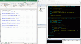
I have reviewed your requirements and demonstrated the situation. I am delighted to inform you that I have developed a solution by creating an Excel VBA Sub-procedure to fulfil your goal.

Demonstrated Dataset:

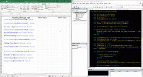
SOLUTION Overview:

Output of running the solution sub-procedure.gif

Excel VBA Sub-procedure:

Code:

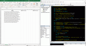
Sub ProcessBaseballData()
    
    Dim ws, wsTMS As Worksheet
    Dim selectedRange As Range
    Dim i As Long
    Dim teamSymbolDict As Object
    
    Set ws = ThisWorkbook.Worksheets("SKD DOG")
    Set wsTMS = ThisWorkbook.Worksheets("TMS")
    
    Set selectedRange = Application.Selection
    
    If selectedRange.Columns.Count > 1 Then
        MsgBox "More than one column has been selected.", vbCritical
        Exit Sub
    End If
    
    Set teamSymbolDict = CreateObject("Scripting.Dictionary")
    Dim teamSymbolRange As Range
    Set teamSymbolRange = wsTMS.ListObjects("TMSYMBOL").DataBodyRange

    Dim teamIndex As Long
    For teamIndex = 1 To teamSymbolRange.Rows.Count
        teamSymbolDict.Add teamSymbolRange.Cells(teamIndex, 1).Value, teamSymbolRange.Cells(teamIndex, 2).Value
    Next teamIndex
    
    For Each cell In selectedRange
        
        If cell.Value = "" Then
            GoTo endOfALoop
        End If
        
        Dim visitorTeam As String
        visitorTeam = Left(cell.Value, InStr(cell.Value, "(") - 2)
        
        Dim visitorSymbol As String
        visitorSymbol = teamSymbolDict(visitorTeam)
        
        ws.Range("C" & cell.Row).Value = visitorSymbol
        
        Dim visitorScore As Integer
        visitorScore = Val(Mid(cell.Value, InStr(cell.Value, "(") + 1, 1))
        
        ws.Range("D" & cell.Row).Value = visitorScore
        
        Dim homeTeam As String
        Dim secondOccurance As Long
        
        secondOccurance = InStr(cell.Value, "(")
        secondOccurance = InStr(secondOccurance + 1, cell.Value, "(")
        
        homeTeam = Trim(Mid(cell.Value, InStr(cell.Value, "@") + 2, secondOccurance - InStr(cell.Value, "@") - 2))
        
        If Left(homeTeam, 1) = " " Then
            homeTeam = Mid(homeTeam, 2)
        End If
        
        Dim homeSymbol As String
        homeSymbol = teamSymbolDict(homeTeam)
        
        ws.Range("H" & cell.Row).Value = homeSymbol
        
        Dim homeScore As Integer
        Dim secondOccuranceNext As Long
        
        secondOccuranceNext = InStr(cell.Value, ")")
        secondOccuranceNext = InStr(secondOccurance + 1, cell.Value, ")")
        
        homeScore = Val(Mid(cell.Value, secondOccurance + 1, secondOccuranceNext - secondOccurance))
        
        ws.Range("I" & cell.Row).Value = homeScore
        
endOfALoop:
        
    Next cell
    
End Sub

Hopefully, you have found the code helpful. I have attached the solution workbook; good luck.

Regards
Lutfor Rahman Shimanto
Excel & VBA Developer
ExcelDemy

Boy282828 · Apr 1, 2024

Dear Lutfor,

Thank you for your prompt response of the VBA to populate Baseball Teams and Scores

into the expected Columns. I deeply appreciate it. There is one catch: when I run the

provided VBA code, it will NOT show the Home Team 3 Letter Symbol in Column H,

all other Visitor Team 3 Letter Symbol, Visitor Team Scores, Home Team Scores are

shown as expected. The reason is the Original Baseball Games and Scores downloaded

from the Internet, between the Home team Score right side bracket “ ) “and the “Boxscore”

tails there is 6 Empty Spaces Positions, when I copy the Games and Scores Assay to the

Thread, it automatically corrects to only 1 space position between all characters, you will

not see the original 6 Empty Spaces Positions, it is my fault that I did not know it. Here is

the Original Games and Score with 6 Empty Spaces Positions:

Colorado Rockies (1) @ Arizona D'Backs (16) Boxscore

Los Angeles Angels (3) @ Baltimore Orioles (11) Boxscore

Detroit Tigers (1) @ Chicago White Sox (0) Boxscore

Washington Nationals (2) @ Cincinnati Reds (8) Boxscore

New York Yankees (5) @ Houston Astros (4) Boxscore

Minnesota Twins (4) @ Kansas City Royals (1) Boxscore

St. Louis Cardinals (1) @ Los Angeles Dodgers (7) Boxscore

Pittsburgh Pirates (6) @ Miami Marlins (5) Boxscore

Cleveland Guardians (8) @ Oakland Athletics (0) Boxscore

San Francisco Giants (4) @ San Diego Padres (6) Boxscore

Boston Red Sox (6) @ Seattle Mariners (4) Boxscore

Toronto Blue Jays (8) @ Tampa Bay Rays (2) Boxscore

Chicago Cubs (3) @ Texas Rangers (4) Boxscore

I suppose on the Thread you can see only 1 space between all Characters.

Could you modify the VBA Code so that the 3 Letter Symbols of the Home

Team Names in Column H will show up? Thanks,

Boy282828 4/1/2024

Lutfor Rahman Shimanto · Apr 2, 2024

Boy282828 said:
Dear Lutfor,

Thank you for your prompt response of the VBA to populate Baseball Teams and Scores

into the expected Columns. I deeply appreciate it. There is one catch: when I run the

provided VBA code, it will NOT show the Home Team 3 Letter Symbol in Column H,

all other Visitor Team 3 Letter Symbol, Visitor Team Scores, Home Team Scores are

shown as expected. The reason is the Original Baseball Games and Scores downloaded

from the Internet, between the Home team Score right side bracket “ ) “and the “Boxscore”

tails there is 6 Empty Spaces Positions, when I copy the Games and Scores Assay to the

Thread, it automatically corrects to only 1 space position between all characters, you will

not see the original 6 Empty Spaces Positions, it is my fault that I did not know it. Here is

the Original Games and Score with 6 Empty Spaces Positions:

Colorado Rockies (1) @ Arizona D'Backs (16) Boxscore

Los Angeles Angels (3) @ Baltimore Orioles (11) Boxscore

Detroit Tigers (1) @ Chicago White Sox (0) Boxscore

Washington Nationals (2) @ Cincinnati Reds (8) Boxscore

New York Yankees (5) @ Houston Astros (4) Boxscore

Minnesota Twins (4) @ Kansas City Royals (1) Boxscore

St. Louis Cardinals (1) @ Los Angeles Dodgers (7) Boxscore

Pittsburgh Pirates (6) @ Miami Marlins (5) Boxscore

Cleveland Guardians (8) @ Oakland Athletics (0) Boxscore

San Francisco Giants (4) @ San Diego Padres (6) Boxscore

Boston Red Sox (6) @ Seattle Mariners (4) Boxscore

Toronto Blue Jays (8) @ Tampa Bay Rays (2) Boxscore

Chicago Cubs (3) @ Texas Rangers (4) Boxscore

I suppose on the Thread you can see only 1 space between all Characters.

Could you modify the VBA Code so that the 3 Letter Symbols of the Home

Team Names in Column H will show up? Thanks,

Boy282828 4/1/2024

Dear, thanks for clarifying the original baseball games and scores downloaded online. You have mentioned that all other Visitor Team 3 Letter Symbols, Visitor Team Scores, and Home Team Scores are displayed as expected. But on your machine, the sub-procedure is not displaying the Home Team 3 Letter Symbol in Column H. In my view, 6 empty spaces are not the reason for not correctly showing the Home Team symbol.

However, I have made the necessary changes to improve the sub-procedure to overcome the problem. Let us know if you are still facing the issue. When you encounter the problem again, we recommend sharing your Excel file within this thread.

OUTPUT Overview:

Improved Excel VBA Sub-procedure:

Code:

Sub AdvancedProcessBaseballData()
    
    Dim ws, wsTMS As Worksheet
    Dim selectedRange As Range
    Dim i As Long
    Dim teamSymbolDict As Object
    
    Set ws = ThisWorkbook.Worksheets("SKD DOG")
    Set wsTMS = ThisWorkbook.Worksheets("TMS")
    
    Set selectedRange = Application.Selection
    
    If selectedRange.Columns.Count > 1 Then
        MsgBox "More than one column has been selected.", vbCritical
        Exit Sub
    End If
    
    Set teamSymbolDict = CreateObject("Scripting.Dictionary")
    Dim teamSymbolRange As Range
    Set teamSymbolRange = wsTMS.ListObjects("TMSYMBOL").DataBodyRange

    Dim teamIndex As Long
    For teamIndex = 1 To teamSymbolRange.Rows.Count
        teamSymbolDict.Add teamSymbolRange.Cells(teamIndex, 1).Value, teamSymbolRange.Cells(teamIndex, 2).Value
    Next teamIndex
    
    For Each cell In selectedRange
        
        If cell.Value = "" Then
            GoTo endOfALoop
        End If
                
        Dim visitorTeam As String
        visitorTeam = Trim(Left(cell.Value, InStr(cell.Value, "(") - 1))
        
        Dim visitorSymbol As String
        visitorSymbol = teamSymbolDict(visitorTeam)
        
        ws.Range("C" & cell.Row).Value = visitorSymbol
        
        Dim visitorScore As Integer
        visitorScore = Val(Mid(cell.Value, InStr(cell.Value, "(") + 1, InStr(cell.Value, ")") - InStr(cell.Value, "(") - 1))
        
        ws.Range("D" & cell.Row).Value = visitorScore
        
        Dim homeTeam As String
        Dim secondOccurance As Long
        
        secondOccurance = InStr(cell.Value, "(")
        secondOccurance = InStr(secondOccurance + 1, cell.Value, "(")
        
        homeTeam = Trim(Mid(cell.Value, InStr(cell.Value, "@") + 1, secondOccurance - InStr(cell.Value, "@") - 1))
        
        Dim homeSymbol As String
        homeSymbol = teamSymbolDict(homeTeam)
        
        ws.Range("H" & cell.Row).Value = homeSymbol
        
        Dim homeScore As Integer
        Dim secondOccuranceNext As Long
        
        secondOccuranceNext = InStr(cell.Value, ")")
        secondOccuranceNext = InStr(secondOccurance + 1, cell.Value, ")")
        
        homeScore = Val(Mid(cell.Value, secondOccurance + 1, secondOccuranceNext - secondOccurance))
        
        ws.Range("I" & cell.Row).Value = homeScore
        
endOfALoop:
        
    Next cell
    
End Sub

Hopefully, the code will fulfil your goal; good luck.

Regards
Lutfor Rahman Shimanto
Excel & VBA Developer
ExcelDemy

Boy282828 · Apr 2, 2024

Dear Lutfor,

I did not get the Luck. When I run the “AdvancedProcesBaseballData” VBA,

Both Column C 3 Letter Symbol of the Visitor Team and Column H 3 Letter Symbol

of the Home Team are gone, the good news is both Visitor & Home team scores are

shown on Column D & Column I as expected.

Since I know how to use Microsoft Built-in Text to Column Function as Array,

I already separate the many terms in the original Column C data. It becomes

For example, like this:

Column C contains “Colorado Rockies (1)”, Array of 2 Terms cells only.

Column H contains “Arizona D'Backs (16) Boxscore”, Array of 3 Terms cells with

Unwanted “Boxscore” Tails.

Could you write 2 VBA Code separately, one is called “VTMS” which means Visitor

TeamNames and Scores so that once I click the Column C selected array, it will convert

Column C to 3 Letter Team Symbol, and in Column D it will show a vertical array which

is a Positive Integer Array without Backet to avoid misunderstand of Negative Number.

Another VBA Code is called “HTMS” which means Home TeamNames and Scores so

that once I click the Column H selected array, it will convert Column H to a 3 Letter

Team Symbol, and in Column I it will show Positive Integer Array without Brackets

and get rid of the unwanted “Boxscore” tails.

Maybe this way it is easier than modifying your VBA Code again? No matter what

way you choose, I respect your decision. Thanks,

Boy282828 4/2/2024

Lutfor Rahman Shimanto · Apr 2, 2024

Boy282828 said:
Dear Lutfor,

I did not get the Luck. When I run the “AdvancedProcesBaseballData” VBA,

Both Column C 3 Letter Symbol of the Visitor Team and Column H 3 Letter Symbol

of the Home Team are gone, the good news is both Visitor & Home team scores are

shown on Column D & Column I as expected.

Since I know how to use Microsoft Built-in Text to Column Function as Array,

I already separate the many terms in the original Column C data. It becomes

For example, like this:

Column C contains “Colorado Rockies (1)”, Array of 2 Terms cells only.

Column H contains “Arizona D'Backs (16) Boxscore”, Array of 3 Terms cells with

Unwanted “Boxscore” Tails.

Could you write 2 VBA Code separately, one is called “VTMS” which means Visitor

TeamNames and Scores so that once I click the Column C selected array, it will convert

Column C to 3 Letter Team Symbol, and in Column D it will show a vertical array which

is a Positive Integer Array without Backet to avoid misunderstand of Negative Number.

Another VBA Code is called “HTMS” which means Home TeamNames and Scores so

that once I click the Column H selected array, it will convert Column H to a 3 Letter

Team Symbol, and in Column I it will show Positive Integer Array without Brackets

and get rid of the unwanted “Boxscore” tails.

Maybe this way it is easier than modifying your VBA Code again? No matter what

way you choose, I respect your decision. Thanks,

Boy282828 4/2/2024

Dear, thanks for your patience. As mentioned, I can develop two individual sub-procedures for the Home and Visitor teams. However, I think the existing code is powerful enough to complete all the required tasks. After you download your Excel data from another website, share a screenshot of it. After reviewing the data, it will be easy to improve the existing code.

Regards
Lutfor Rahman Shimanto
ExcelDemy

Boy282828 · Apr 2, 2024

Dear Lutfor,

The original MLB Baseball Schedule and Scores is from this Website:

https://www.baseball-reference.com/leagues/MLB-schedule.shtml

I hope you can open it and see the data I copy and paste to your place.

I never know how to make “Screenshot”, if you can see the data, it will

save me lots of time trying to search the Internet learning how to do it.

Thanks,

Boy282828 4/2/2024

Lutfor Rahman Shimanto · Apr 3, 2024

Boy282828 said:
Dear Lutfor,

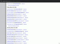
The original MLB Baseball Schedule and Scores is from this Website:

https://www.baseball-reference.com/leagues/MLB-schedule.shtml

I hope you can open it and see the data I copy and paste to your place.

I never know how to make “Screenshot”, if you can see the data, it will

save me lots of time trying to search the Internet learning how to do it.

Thanks,

Boy282828 4/2/2024

Dear, Thanks for providing the link to the original MLB Baseball Schedule and Scores Website. I am delighted to inform you that I have overcome your situation with the help of two more VBA User-defined functions and the improved VBA Sub-procedure.

SOLUTION Overview:

Copying Data from Website:
Running Excel VBA Solution Sub-procedure:

SOLUTION Excel VBA Code:

Code:

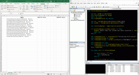
Sub AdvancedProcessBaseballData()
    
    Dim ws, wsTMS As Worksheet
    Dim selectedRange As Range
    Dim i As Long
    Dim teamSymbolDict As Object
    
    Set ws = ThisWorkbook.Worksheets("SKD DOG")
    Set wsTMS = ThisWorkbook.Worksheets("TMS")
    
    Set selectedRange = Application.Selection
    
    If selectedRange.Columns.Count > 1 Then
        MsgBox "More than one column has been selected.", vbCritical
        Exit Sub
    End If
    
    Set teamSymbolDict = CreateObject("Scripting.Dictionary")
    Dim teamSymbolRange As Range
    Set teamSymbolRange = wsTMS.ListObjects("TMSYMBOL").DataBodyRange

    Dim teamIndex As Long
    For teamIndex = 1 To teamSymbolRange.Rows.Count
        teamSymbolDict.Add teamSymbolRange.Cells(teamIndex, 1).Value, teamSymbolRange.Cells(teamIndex, 2).Value
    Next teamIndex
    
    For Each cell In selectedRange
        
        If cell.Value = "" Then
            GoTo endOfALoop
        End If
                
        cell.Value = ReplaceChar(cell.Value)
                
        Dim visitorTeam As String
        visitorTeam = Left(cell.Value, InStr(cell.Value, "(") - 1)
        
        visitorTeam = TrimSpaces(visitorTeam)
        
        Dim visitorSymbol As String
        visitorSymbol = teamSymbolDict(visitorTeam)
        
        ws.Range("C" & cell.Row).Value = visitorSymbol
        
        Dim visitorScore As Integer
        visitorScore = Val(Mid(cell.Value, InStr(cell.Value, "(") + 1, InStr(cell.Value, ")") - InStr(cell.Value, "(") - 1))
        
        ws.Range("D" & cell.Row).Value = visitorScore
        
        Dim homeTeam As String
        Dim secondOccurance As Long
        
        secondOccurance = InStr(cell.Value, "(")
        secondOccurance = InStr(secondOccurance + 1, cell.Value, "(")
        
        homeTeam = Mid(cell.Value, InStr(cell.Value, "@") + 1, secondOccurance - InStr(cell.Value, "@") - 1)
        
        homeTeam = TrimSpaces(homeTeam)
        
        Dim homeSymbol As String
        homeSymbol = teamSymbolDict(homeTeam)
        
        ws.Range("H" & cell.Row).Value = homeSymbol
        
        Dim homeScore As Integer
        Dim secondOccuranceNext As Long
        
        secondOccuranceNext = InStr(cell.Value, ")")
        secondOccuranceNext = InStr(secondOccurance + 1, cell.Value, ")")
        
        homeScore = Val(Mid(cell.Value, secondOccurance + 1, secondOccuranceNext - secondOccurance))
        
        ws.Range("I" & cell.Row).Value = homeScore
        
endOfALoop:
        
    Next cell
    
End Sub

Function TrimSpaces(ByVal inputString As String) As String

    While Left(inputString, 1) = " "
        inputString = Right(inputString, Len(inputString) - 1)
    Wend

    While Right(inputString, 1) = " "
        inputString = Left(inputString, Len(inputString) - 1)
    Wend

    TrimSpaces = inputString

End Function

Function ReplaceChar(ByVal inputString As String) As String

    Dim resultString As String
    Dim i As Integer
    Dim charCode As Integer
    
    For i = 1 To Len(inputString)

        charCode = Asc(Mid(inputString, i, 1))
        
        If charCode = 160 Then
            resultString = resultString & " "
        Else
            resultString = resultString & Mid(inputString, i, 1)
        End If
    Next i

    ReplaceChar = resultString

End Function

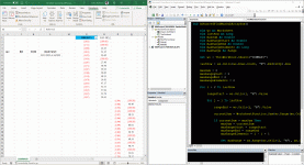
Initial Problem: You are right about the problem when you have copied data from the website.

Initial problem of putting daily MLB Baseball Games results in Excel using VBA Code.gif

SOLUTION: Websites sometimes use non-breaking spaces to maintain formatting. These spaces look like regular spaces, but VBA treats them differently. A regular space will have a code of 32, while a non-breaking space might have a different code. Using Asc functions in VBA, I checked all the character codes for each cell. I also found that all the non-breaking spaces have an Asc code of 160. That is the key to overcoming the problem. Later, I replaced these with regular spaces.

Hopefully, you have found an ultimate solution. I have attached the solution workbook used to investigate the problem. Stay connected, and good luck.

Regards
Lutfor Rahman Shimanto
Excel & VBA Developer
ExcelDemy

Boy282828 · Apr 3, 2024

Dear Lutfor,

Thanks for your great help, I run the modified Code in your own Excel

named “2024MLB” it works Perfect, all 4 Columns data shown as expected.

In my own Excel named “2024MLB.xlsm” it won’t work since my Headings

starts on Row# 6, above Row# 6 I wrote a lot of Symbols with respect to

how to use it in Microsoft Built-in Functions, plus Statistical Facts of

Last year’s MLB Baseball results, I just can’t erase them. If I run it, the

Run-Time Bug show up stating some Code Line “Subject out of range”,

so I Rename your own Excel to “2024MLBEXCELDEMY.xlsm”, run it

and Copy/Paste the desired results to my “2024MLB.xlsm” Workbook.

Since I achieved my goal, you don’t have to examine my Workbook

to find the hidden “Secrets” only Professional Software Engineer knows

to save your precious time. The Problem has been resolved. You can close

this Case now. Your fast and kind help is deeply appreciated. Thanks,

Boy282828 4/3/2024

Lutfor Rahman Shimanto · Apr 4, 2024

Boy282828 said:
Dear Lutfor,

Thanks for your great help, I run the modified Code in your own Excel

named “2024MLB” it works Perfect, all 4 Columns data shown as expected.

In my own Excel named “2024MLB.xlsm” it won’t work since my Headings

starts on Row# 6, above Row# 6 I wrote a lot of Symbols with respect to

how to use it in Microsoft Built-in Functions, plus Statistical Facts of

Last year’s MLB Baseball results, I just can’t erase them. If I run it, the

Run-Time Bug show up stating some Code Line “Subject out of range”,

so I Rename your own Excel to “2024MLBEXCELDEMY.xlsm”, run it

and Copy/Paste the desired results to my “2024MLB.xlsm” Workbook.

Since I achieved my goal, you don’t have to examine my Workbook

to find the hidden “Secrets” only Professional Software Engineer knows

to save your precious time. The Problem has been resolved. You can close

this Case now. Your fast and kind help is deeply appreciated. Thanks,

Boy282828 4/3/2024

Dear, I am glad that the improved sub-procedure code has worked perfectly so far. Copying the desired results into the "2024 MLB.xlsm" workbook from "2024 MLB EXCELDEMY.xlsm" is an obvious solution. I appreciate naming our provided file "2024MLBEXCELDEMY.xlsm," assuming a creative way of expressing gratitude.

There might be ways to adjust the VBA code to work around the headings in Row #6 without transferring data between workbooks. If you want to explore that option, I will happily improve the VBA code further when handling the specific layout of the "2024MLB.xlsm" file.

However, I completely respect your decision to close the case. Your time is also valuable.

Thank you again for your kind words. I'm always happy to help with VBA!

Regards
Lutfor Rahman Shimanto
ExcelDemy

Boy282828 · Apr 10, 2024

Dear Lutfor,

Last time you help me resolve the update of MLB Baseball Team & Score problem,

using your VBA Code I update all the game scores daily without any problem,

I really appreciate it.

This time I have a new problem and need your help. Enclosed please find my Excel

workbook named “SportsMaxNPRangeLRCharts.xlsm”, before the name hyphen –

is today’s date 04102024, which means 4/10/2024. Currently only 1 worksheet name

“SUMMARY” is created. On this worksheet Column N Head Title is “RDF(H-V)”,

Column O Head Title is “FAV 4W”, below the 2 Column Titles are 2 Real Number

(including negative numbers with decimal points) Vertical Array, they are parallel

with the same row numbers and without any gap or blanks. Each Column has 790

Real Number elements. I need to know at what vertical of SubArray of Column N

Range such that you can get the Maximum Sum of SubArray of Column O with

the same Row Numbers? For example, I guess a vertical SubArray in Column N

from Negative -0.568 to Negative -0.368 Range and add the elements SubArray

in Column O with the same Row numbers, the SUM value is 2079.57. Since

there are too many SubArrays with numbers of elements from 2 to 790, I don’t

think my guess is right. The true Max Sum of SubArray in Column O is hidden

somewhere. Could you write VBA Code to run it, the Message shows something

like “ The SubArray of RDF(H-V) ranges from x (smallest number) to y (largest number)

such that the Max Sum Value is z with u number elements SubArray in FAV 4W ” .

x,y,z,u are calculated results from VBA Calculation. I am curious about the True

Max Sum value in FAV 4W Column O SubArray. Could you run the Code and

Show me the true Max value? The RDF(H-V) Column N is arranged in Ascending

Order from small number to large number, I should mention it earlier. Thanks,

Boy282828 4/10/2024

Lutfor Rahman Shimanto · Apr 16, 2024

Boy282828 said:
Dear Lutfor,

Last time you help me resolve the update of MLB Baseball Team & Score problem,

using your VBA Code I update all the game scores daily without any problem,

I really appreciate it.

This time I have a new problem and need your help. Enclosed please find my Excel

workbook named “SportsMaxNPRangeLRCharts.xlsm”, before the name hyphen –

is today’s date 04102024, which means 4/10/2024. Currently only 1 worksheet name

“SUMMARY” is created. On this worksheet Column N Head Title is “RDF(H-V)”,

Column O Head Title is “FAV 4W”, below the 2 Column Titles are 2 Real Number

(including negative numbers with decimal points) Vertical Array, they are parallel

with the same row numbers and without any gap or blanks. Each Column has 790

Real Number elements. I need to know at what vertical of SubArray of Column N

Range such that you can get the Maximum Sum of SubArray of Column O with

the same Row Numbers? For example, I guess a vertical SubArray in Column N

from Negative -0.568 to Negative -0.368 Range and add the elements SubArray

in Column O with the same Row numbers, the SUM value is 2079.57. Since

there are too many SubArrays with numbers of elements from 2 to 790, I don’t

think my guess is right. The true Max Sum of SubArray in Column O is hidden

somewhere. Could you write VBA Code to run it, the Message shows something

like “ The SubArray of RDF(H-V) ranges from x (smallest number) to y (largest number)

such that the Max Sum Value is z with u number elements SubArray in FAV 4W ” .

x,y,z,u are calculated results from VBA Calculation. I am curious about the True

Max Sum value in FAV 4W Column O SubArray. Could you run the Code and

Show me the true Max value? The RDF(H-V) Column N is arranged in Ascending

Order from small number to large number, I should mention it earlier. Thanks,

Boy282828 4/10/2024

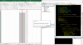
Dear, it is good to see you again. Thanks for sharing your requirements.

You want to find the vertical subarray in Column N, where the sum of the corresponding elements in Column O is maximized. I am delighted to inform you that I have developed an Excel VBA Sub-procedure to fulfil your goal.

SOLUTION Overview:

Excel VBA Sub-procedure:

Code:

Sub AdvancedFindMaxSubArraySum()

    Dim ws As Worksheet
    Dim lastRow As Long
    Dim maxSum As Double
    Dim maxRangeStart As Double
    Dim maxRangeEnd As Double
    Dim maxRangeElements As Long
    Dim maxRange As Range
    
    Set ws = ThisWorkbook.Sheets("SUMMARY")
    
    lastRow = ws.Cells(ws.Rows.Count, "N").End(xlUp).Row
    
    maxSum = 0
    maxRangeStart = 0
    maxRangeEnd = 0
    maxRangeElements = 0
    
    For i = 2 To lastRow

        rangeStart = ws.Cells(i, "N").Value
        
        For j = i To lastRow

            rangeEnd = ws.Cells(j, "N").Value
            
            currentSum = WorksheetFunction.Sum(ws.Range(ws.Cells(i, "O"), ws.Cells(j, "O")))
            
            If currentSum > maxSum Then
                maxSum = currentSum
                maxRangeStart = rangeStart
                maxRangeEnd = rangeEnd
                maxRangeElements = j - i + 1

                Set maxRange = ws.Range(ws.Cells(i, "N"), ws.Cells(j, "N"))
            End If
        Next j
    Next i
    
    MsgBox "The SubArray of RDF(H-V) ranges from " & maxRangeStart & " to " & maxRangeEnd & " such that the Max Sum Value is " & maxSum & " with " & maxRangeElements & " number elements SubArray in FAV 4W."
    
    If Not maxRange Is Nothing Then
        maxRange.Select
    End If

End Sub

NOTE: Additionally, I have added some extra lines of code to select the ranges for my testing purposes. You can turn these lines of code into comments or remove these lines.

A Friendly Suggestion: It would be great to post the problem by creating a new thread, as it differs from the previous one.

I have attached the workbook used to investigate your problem; good luck.

Regards
Lutfor Rahman Shimanto
Excel & VBA Developer
ExcelDemy

Boy282828 · Apr 16, 2024

Dear Lutfor,

I am glad to chat with you again. I am sorry that I did not know I should create a

new Post of new Problem, is that true to create new problem next time, I go from

the menu “Forums” then go to “New Posts” to create new thread? I post the new

problem on old thread on 4/10/2024, I am in no hurry and thought maybe you are

too busy to answer my question, it is all my fault. By running the VBA Code you

provided, I got confused because all the real numbers have 16 digit decimal points,

the Second answer is in Scientific Exponential Mode 16 digit decimal point, which

I misinterpreted it as “-1.110” instead of the real 3 digit Number “-0.011”.

Could you modify the Message such that the 1st and the 2nd real numbers have

3 digit decimal point numbers, and the 3rd real number has 2 digit decimal points

which are consistent with the original Column Formatting. That is, the Message

print out should be like this:

“The SubArray in RDF(H-V) ranges from -0.568 to -0.011 such that that the Max Sum Value is 2311.78 with 159 elements SubArray in FAV 4W.”

Besides the above, every time I download your Excel, Microsoft will block the

VBA Code stating that it is “Untrusted”, it is a headache for me to ask Google

to Unblock the Code, could you show me how to tell Microsoft that as long as

I get any Excel from your ExcelDemy Website, all VBA Codes can be trusted

and unblocked? How to put your website on the Unblock list? Thanks,

Boy282828 4/16/2024

Boy282828 · Apr 16, 2024

Dear Lutfor,

I am glad to chat with you again. I am sorry that I did not know I should create a

new Post of new Problem, is that true to create new problem next time, I go from

the menu “Forums” then go to “New Posts” to create new thread? I post the new

problem on old thread on 4/10/2024, I am in no hurry and thought maybe you are

too busy to answer my question, it is all my fault. By running the VBA Code you

provided, I got confused because all the real numbers have 16 digit decimal points,

the Second answer is in Scientific Exponential Mode 16 digit decimal point, which

I misinterpreted it as “-1.110” instead of the real 3 digit Number “-0.011”.

Could you modify the Message such that the 1st and the 2nd real numbers have

3 digit decimal point numbers, and the 3rd real number has 2 digit decimal points

which are consistent with the original Column Formatting. That is, the Message

print out should be like this:

“The SubArray in RDF(H-V) ranges from -0.568 to -0.011 such that that the Max Sum Value is 2311.78 with 159 elements SubArray in FAV 4W.”

Besides the above, every time I download your Excel, Microsoft will block the

VBA Code stating that it is “Untrusted”, it is a headache for me to ask Google

to Unblock the Code, could you show me how to tell Microsoft that as long as

I get any Excel from your ExcelDemy Website, all VBA Codes can be trusted

and unblocked? How to put your website on the Unblock list? Thanks,

Boy282828 4/16/2024

Lutfor Rahman Shimanto · Apr 21, 2024

Boy282828 said:
Dear Lutfor,

I am glad to chat with you again. I am sorry that I did not know I should create a

new Post of new Problem, is that true to create new problem next time, I go from

the menu “Forums” then go to “New Posts” to create new thread? I post the new

problem on old thread on 4/10/2024, I am in no hurry and thought maybe you are

too busy to answer my question, it is all my fault. By running the VBA Code you

provided, I got confused because all the real numbers have 16 digit decimal points,

the Second answer is in Scientific Exponential Mode 16 digit decimal point, which

I misinterpreted it as “-1.110” instead of the real 3 digit Number “-0.011”.

Could you modify the Message such that the 1st and the 2nd real numbers have

3 digit decimal point numbers, and the 3rd real number has 2 digit decimal points

which are consistent with the original Column Formatting. That is, the Message

print out should be like this:

“The SubArray in RDF(H-V) ranges from -0.568 to -0.011 such that that the Max Sum Value is 2311.78 with 159 elements SubArray in FAV 4W.”

Besides the above, every time I download your Excel, Microsoft will block the

VBA Code stating that it is “Untrusted”, it is a headache for me to ask Google

to Unblock the Code, could you show me how to tell Microsoft that as long as

I get any Excel from your ExcelDemy Website, all VBA Codes can be trusted

and unblocked? How to put your website on the Unblock list? Thanks,

Boy282828 4/16/2024

Hello Dear

It is great to chat with you as well. Thanks for staying with ExcelDemy Forum and considering ExcelDemy as your trusted website. We appreciate your concern. Unfortunately, there is no way to trust all VBA code downloaded from a specific website globally.

Do not worry! I have come up with an alternative solution. All you have to do is create a folder named ExcelDemy (you can give it any name you want) and then make this a trusted location. Now, you can keep all the Excel files downloaded from the ExcelDemy Website within the ExcelDemy folder (created by you). As a result, you will be able to open and use all files within the ExcelDemy folder without unblocking these files.

Open the Microsoft Excel >> Options >> Trust Center >> Trust Center Settings >> Trusted Location >> Add new location >> Browse (Choose the folder named ExcelDemy) >> [OK >> OK >> OK] (from 3 different dialogue boxes).

Now, let us discuss how your message displays according to your mentioned requirements. I applied formatting to fulfil your goal, that's all.

OUTPUT Overview:

Displaying 1st and 2nd Real numbers with 3-digit decimal point and the 3rd Real number with 2-...png

Excel VBA Sub-procedure:

Code:

Sub AdvancedFindMaxSubArraySum()

    Dim ws As Worksheet
    Dim lastRow As Long
    Dim maxSum As Double
    Dim maxRangeStart As Double
    Dim maxRangeEnd As Double
    Dim maxRangeElements As Long
    Dim maxRange As Range
    
    Set ws = ThisWorkbook.Sheets("SUMMARY")
    
    lastRow = ws.Cells(ws.Rows.Count, "N").End(xlUp).Row
    
    maxSum = 0
    maxRangeStart = 0
    maxRangeEnd = 0
    maxRangeElements = 0
    
    For i = 2 To lastRow

        rangeStart = ws.Cells(i, "N").Value
        
        For j = i To lastRow

            rangeEnd = ws.Cells(j, "N").Value
            
            currentSum = WorksheetFunction.Sum(ws.Range(ws.Cells(i, "O"), ws.Cells(j, "O")))
            
            If currentSum > maxSum Then
                maxSum = currentSum
                maxRangeStart = rangeStart
                maxRangeEnd = rangeEnd
                maxRangeElements = j - i + 1

                Set maxRange = ws.Range(ws.Cells(i, "N"), ws.Cells(j, "N"))
            End If
        Next j
    Next i
    
    MsgBox "The SubArray in RDF(H-V) ranges from " & Format(maxRangeStart, "0.000") & " to " & Format(maxRangeEnd, "0.000") & " such that the Max Sum Value is " & Format(maxSum, "0.00") & " with " & maxRangeElements & " elements SubArray in FAV 4W."
    
    If Not maxRange Is Nothing Then
        maxRange.Select
    End If

End Sub

I hope you have found the ideas helpful and like the solution. I have attached the solution workbook. Stay blessed.

Regards
Lutfor Rahman Shimanto
Excel & VBA Developer
ExcelDemy

Boy282828 · Apr 25, 2024

Dear Lutfor,

I created a folder named ExcelDemy per your instruction procedures,

run the revised Code, got the expected results successfully. Thanks.

Next time if new problems, I will create a new thread per your advice.

Can I report my findings of MLB Baseball Game results just for fun?

If you think it is not related to VBA Code violating your website rules,

I respect your decision not to mention anything else. What do you think?

Boy282828 4/24/2024

Lutfor Rahman Shimanto · Apr 25, 2024

Boy282828 said:
Dear Lutfor,

I created a folder named ExcelDemy per your instruction procedures,

run the revised Code, got the expected results successfully. Thanks.

Next time if new problems, I will create a new thread per your advice.

Can I report my findings of MLB Baseball Game results just for fun?

If you think it is not related to VBA Code violating your website rules,

I respect your decision not to mention anything else. What do you think?

Boy282828 4/24/2024

Dear, It is great to know that the solution worked perfectly on your end and successfully achieved the expected result. Thanks for thanking me; you are welcome.

We really appreciate your thoughts about creating new threads for new problems. I would say it is very visitor-friendly, as many visitors come here and learn various practical problems by reading these threads.

Absolutely, I am really interested to know about your issues and findings on the MLB Baseball Game result.

Regards
Lutfor Rahman Shimanto
ExcelDemy

COL	1	ARI	16
LAA	3	BAL	11
DET	1	CHW	0
WAS	2	CIN	8
NYY	5	HOU	4
MIN	4	KC	1
STL	1	LAD	7
PIT	6	MIA	5
CLE	8	OAK	0
SF	4	SD	6
BOS	6	SF	4
TOR	8	TB	2
CHC	3	TEX	4

COL	1	ARI	16
LAA	3	BAL	11
DET	1	CHW	0
WAS	2	CIN	8
NYY	5	HOU	4
MIN	4	KC	1
STL	1	LAD	7
PIT	6	MIA	5
CLE	8	OAK	0
SF	4	SD	6
BOS	6	SF	4
TOR	8	TB	2
CHC	3	TEX	4

How to put daily MLB Baseball Games results in Excel using VBA Code?

New member

Active member

Attachments

New member

Active member

New member

Active member

New member

Active member

Attachments

New member

Active member

New member

Attachments

Active member

Attachments

New member

New member

Active member

Attachments

New member

Active member

Online statistics

Forum statistics

Share this page

COL	1	ARI	16
LAA	3	BAL	11
DET	1	CHW	0
WAS	2	CIN	8
NYY	5	HOU	4
MIN	4	KC	1
STL	1	LAD	7
PIT	6	MIA	5
CLE	8	OAK	0
SF	4	SD	6
BOS	6	SF	4
TOR	8	TB	2
CHC	3	TEX	4