I have followed the instructions in How To Create a Credit Card Payment sheet and everything is working except that the rows are not hidden if the value in column b is empty. This is because the tutorial uses the Sequence function and my version of Excel does not allow the sequence function. Therefore, the VBA code that is inserted in the spreadsheet is not working. Is there a way around this or am I just stuck with what I have? Great tutorial by the way.
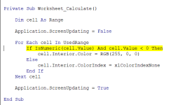
Also, I can't seem to figure out how to display cells in red background if the value is a negative number.
Also, I can't seem to figure out how to display cells in red background if the value is a negative number.
Last edited: