[Solved] Auto populate Task to calendar

2018acway

New member
Good day,

I'm looking for help with a formula. I have a bunch of tasks that fall on certain days. I want a formula to plan it onto an instructor that has
the skill.

Tasks are located on the third tab marked Master List. Sheet2 has my instructor's skills.

I currently have to manually plan the tasks onto the Master tab. I would like to see a formula that auto plans tasks.
 

Attachments

Good day,

I'm looking for help with a formula. I have a bunch of tasks that fall on certain days. I want a formula to plan it onto an instructor that has
the skill.

Tasks are located on the third tab marked Master List. Sheet2 has my instructor's skills.

I currently have to manually plan the tasks onto the Master tab. I would like to see a formula that auto plans tasks.
Dear, Thanks for explaining your requirements further! I have reviewed your problem and created two complex formulas: one for populating training and course codes and another for shift times.

To develop formulas that would fulfil your goal, I used the IFERROR, TEXTJOIN, TRANSPOSE, FILTER, FIND, UPPER, and MID functions.

Populating Traning and Course Codes:
  1. Select the intended cell.
  2. Apply the following formula:
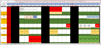
    =IFERROR(TEXTJOIN(", ",TRUE,TRANSPOSE(FILTER('Master List'!$A$3:$A$202& " " & 'Master List'!$F$3:$F$202,('Master List'!$C$3:$C$202=Master!CV$2)*IFERROR(FIND(UPPER(MID(Master!$A$5, 1, FIND(" ", Master!$A$5)-1)), 'Master List'!$G$3:$G$202), 0)))),"")
  3. Drag the Fill Handle icon to the right.
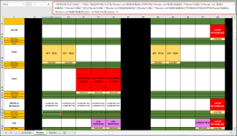
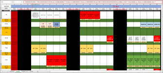
    Populating training and course code in Master sheet.png

Populating Shift Times:
  1. Select the intended cell.
  2. Apply the following formula:
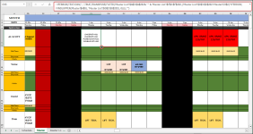
    =IFERROR(TEXTJOIN(", ",TRUE,TRANSPOSE(FILTER('Master List'!$E$3:$E$203,('Master List'!$C$3:$C$203=Master!CV$2)*IFERROR(FIND(UPPER(MID(Master!$A$5, 1, FIND(" ", Master!$A$5)-1)), 'Master List'!$G$3:$G$203), 0)))),"")
  3. Drag the Fill Handle icon to the right.
    Populating shift times in Master sheet.png

I have attached the solution workbook for better understanding; good luck.

Regards
Lutfor Rahman Shimanto
ExcelDemy
 

Attachments

Thank you, again. Is there a way to divide the task between the instructors that have the skills? and can it plan task to run from a set date. Let's say April first we have 8 tasks that start on April 1 and end on April 5th. Can a formula be created to plan that and to separate the tasks?
 
Good day, I've been trying to use this formula. The issue is that if I take away a skill. The Master doesn't not update. Example - On Apr 2nd on AL's line it shows cnx. If I take away that skill from him. The task still shows on Apr 2nd
 
Good day, I've been trying to use this formula. The issue is that if I take away a skill. The Master doesn't not update. Example - On Apr 2nd on AL's line it shows cnx. If I take away that skill from him. The task still shows on Apr 2nd
Dear, Thanks for your patience! I have reviewed the problem you mentioned. You are right! The reason behind this is that your data is not consistent. To overcome this situation, it is recommended that you insert the full name of an instructor in the Master sheet.

Don't worry! I have improved the previously given formulas, and they work fine. You only need to put the instructor's full name instead of using any short name or code name.

Populating Traning and Course Codes:
  1. Select the intended cell.
  2. Apply the following formula:
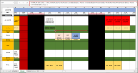
    =IFERROR(TEXTJOIN(", ",TRUE,TRANSPOSE(FILTER('Master List'!$A$3:$A$202& " " & 'Master List'!$F$3:$F$202,('Master List'!$C$3:$C$202=Master!CV$2)*IFERROR(FIND(UPPER(Master!$A$5), 'Master List'!$G$3:$G$202), 0)))),"")
  3. Drag the Fill Handle icon to the right.
    Populating Traning and Course Codes.png

Populating Shift Times:
  1. Select the intended cell.
  2. Apply the following formula:
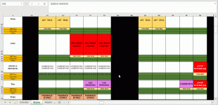
    =IFERROR(TEXTJOIN(", ",TRUE,TRANSPOSE(FILTER('Master List'!$E$3:$E$203,('Master List'!$C$3:$C$203=Master!CV$2)*IFERROR(FIND(UPPER(Master!$A$5), 'Master List'!$G$3:$G$203), 0)))),"")
  3. Drag the Fill Handle icon to the right.
    Populating Shift Times.png

Let me clarify the previous problem. Al is an instructor's name. The algorithm of the last formula tries to find any position that matches the instructor's name within column G in the Master List sheet. So, Al has also been found in the 122nd position of a cell within Mark Falconer.

I hope these formulas will help. Let me see how it goes. I have attached the solution workbook as well. Stay blessed.

Regards
Lutfor Rahman Shimanto
ExcelDemy
 

Attachments

Thank you for your hard work. You are correct AL is an instructor. But when I apply the formula to say Jessica that does not have the skill to do pushbacks, but it comes up that she is qualified. Also, on the Master list "LOADER" task runs from April 1 to the 5th. how can we capture that?
 
Thank you for your hard work. You are correct AL is an instructor. But when I apply the formula to say Jessica that does not have the skill to do pushbacks, but it comes up that she is qualified. Also, on the Master list "LOADER" task runs from April 1 to the 5th. how can we capture that?
Dear, Thanks for your patience! I have reviewed the problem you mentioned. You are right! The reason behind this is that you may have missed making proper cell references for JESSICA HUDSON. When you apply the formulas for a new instructor, you must adjust the formulas. Please check the following:

How to use the complex formulas for a new instructor.gif

Populating Traning and Course Codes:
  1. Select the intended cell.
  2. Apply the following formula:
    =IFERROR(TEXTJOIN(", ",TRUE,TRANSPOSE(FILTER('Master List'!$A$3:$A$202&" "&'Master List'!$F$3:$F$202,IFERROR(('Master List'!$C$3:$C$202<=Master!CV$2)*('Master List'!$D$3:$D$202>=Master!CV$2)*(IF(((Master!CV$2>='Master List'!$C$3:$C$202)*(Master!CV$2<='Master List'!$D$3:$D$202)*IFERROR(FIND(UPPER(Master!$A$30),'Master List'!$G$3:$G$202),0))<>0,TRUE,FALSE)),0)))),"")
  3. Drag the Fill Handle icon to the right.
    Populating Traning and Course Codes.png

Populating Shift Times:
  1. Select the intended cell.
  2. Apply the following formula:
    =IFERROR(TEXTJOIN(", ",TRUE,TRANSPOSE(FILTER('Master List'!$E$3:$E$202,IFERROR(('Master List'!$C$3:$C$202<=Master!CV$2)*('Master List'!$D$3:$D$202>=Master!CV$2)*(IF(((Master!CV$2>='Master List'!$C$3:$C$202)*(Master!CV$2<='Master List'!$D$3:$D$202)*IFERROR(FIND(UPPER(Master!$A$30),'Master List'!$G$3:$G$202),0))<>0,TRUE,FALSE)),0)))),"")
  3. Drag the Fill Handle icon to the right.
    Populating Shift Times.png

I hope these formulas will help. Let me see how it goes. I have attached the solution workbook as well. Good luck.

Regards
Lutfor Rahman Shimanto
ExcelDemy
 

Attachments

Is it too much to ask for the formula to plan only one task in the cell? I would like to see one task assigned and the next task to be assigned to the next available and qualified instructor
 
Is it too much to ask for the formula to plan only one task in the cell? I would like to see one task assigned and the next task to be assigned to the next available and qualified instructor
Dear, Thanks for your query! I have reviewed your dataset and found that merged cells exist. So, if you use an array formula to populate the intended values, you might get a #SPILL! Error. Moreover, developing such formulas would be very time-consuming.

So, I recommend you use the previously given formulas and drag the Fill Handle icon to the right. Good luck.

Regards
Lutfor Rahman Shimanto
ExcelDemy
 

Online statistics

Members online
0
Guests online
1
Total visitors
1

Forum statistics

Threads
352
Messages
1,543
Members
653
Latest member
JeremyTearm
Back
Top