I'm having trouble overlaying data from both solar and usage data for electricity. The problem is that the solar data is measured in 15-minute intervals and the usage data is done by the hour. I have tried to organize the data according to that, but the problem is that the usage data shows up as 1/4th the size of the solar data, and fills the missing data with zeros.
You are using an out of date browser. It may not display this or other websites correctly.
You should upgrade or use an alternative browser.
You should upgrade or use an alternative browser.
[Solved] Condensing Data
- Thread starter tbergines
- Start date
Hello tbergines,
Thanks for reaching us. I understand that you need help organizing data. As the Solar data and Usage data are unequal in size, the missing values are filled by zero.
To solve this problem, we can organize the data in a slightly different manner. From your dataset, I filtered the required values in the following way:
Here, I used the following formula to filter out the required date values:
Afterward, to filter out the time values, I used a similar formula:
However, since the Filter function is only available in MS Office 365, use the following alternative formula if you don’t have access to MS Office 365.
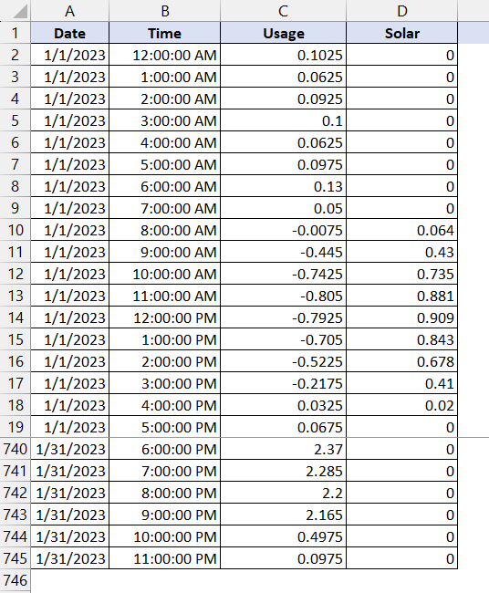
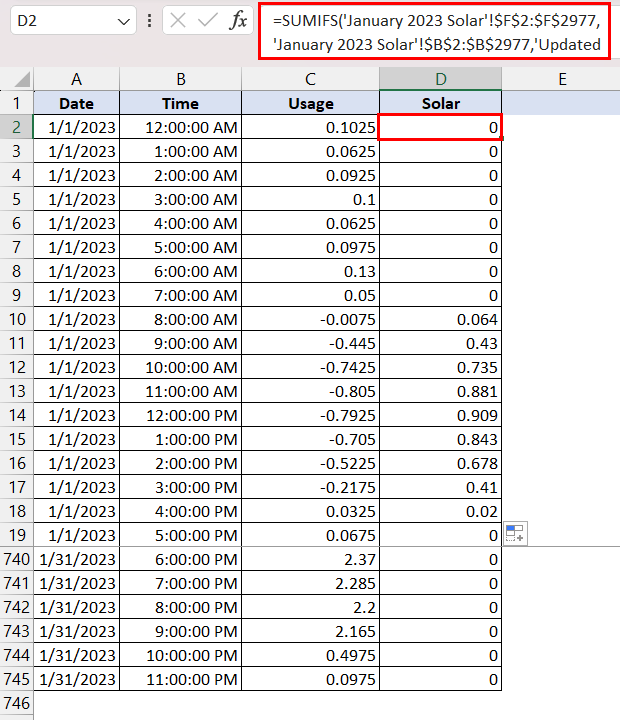
For the Usage data, I copied and pasted the actual non-zero filled values, and for Solar data, I summed all the values with the same Time Interval for each date. I used the following formula to accomplish that:
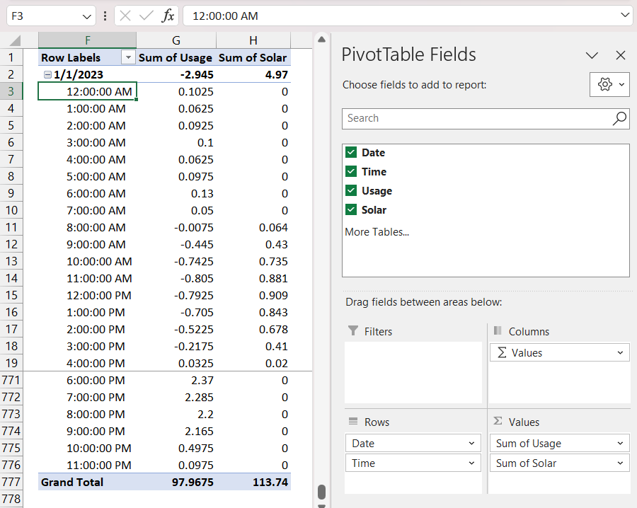
Then I inserted a Pivot Table using this filtered dataset:
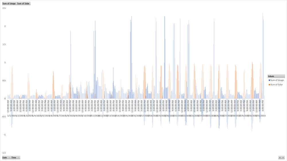
Then I inserted a Pivot Chart-
 The workbook with the updated dataset is attached below.
Hopefully, I was able to resolve your problem. Let us know your feedback.
Regards,
Seemanto Saha
ExcelDemy
Thanks for reaching us. I understand that you need help organizing data. As the Solar data and Usage data are unequal in size, the missing values are filled by zero.
To solve this problem, we can organize the data in a slightly different manner. From your dataset, I filtered the required values in the following way:
Here, I used the following formula to filter out the required date values:
=FILTER('January 2023 Solar'!B2:B2977,MOD(ROW('January 2023 Solar'!B2:B2977)-1,4)=1)
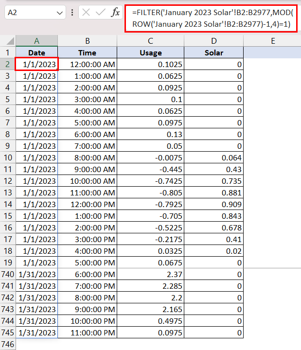
You may require changing the Number Format of these cells to Date.
Afterward, to filter out the time values, I used a similar formula:
=FILTER('January 2023 Solar'!C2:C2977,MOD(ROW('January 2023 Solar'!C2:C2977)-1,4)=1)
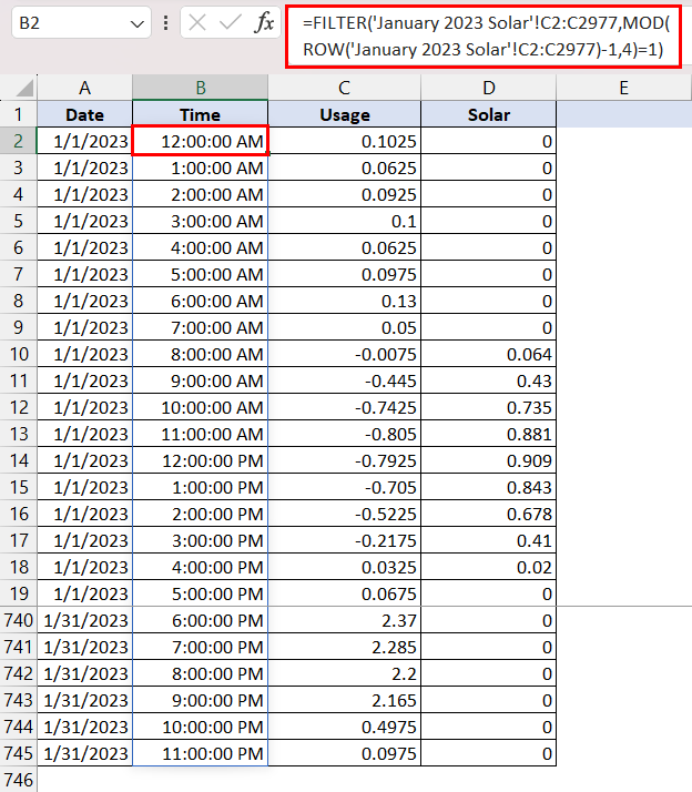
Change the Number Format of these cells to Time if required.
However, since the Filter function is only available in MS Office 365, use the following alternative formula if you don’t have access to MS Office 365.
=TEXT(TEXTSPLIT(TEXTJOIN(",",TRUE,IF(MOD(ROW('January 2023 Solar'!B2:B2977)-1,4)=1,'January 2023 Solar'!B2:B2977,"")),,","),"m/dd/yyyy")
For the Usage data, I copied and pasted the actual non-zero filled values, and for Solar data, I summed all the values with the same Time Interval for each date. I used the following formula to accomplish that:
=SUMIFS('January 2023 Solar'!$F$2:$F$2977,'January 2023 Solar'!$B$2:$B$2977,'Updated Dataset'!A2,'January 2023 Solar'!$C$2:$C$2977,'Updated Dataset'!B2)
Then I inserted a Pivot Table using this filtered dataset:
Then I inserted a Pivot Chart-
Hopefully, I was able to resolve your problem. Let us know your feedback.
Regards,
Seemanto Saha
ExcelDemy