[Solved] Excel LOOKUP Formula Help

[tmbutter]

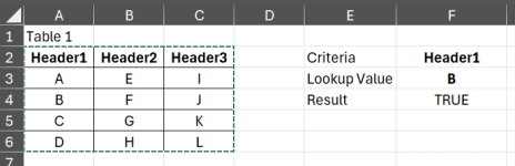
I have a large data set roughly laid out like the below example. I need to filter the see if a specific value (ex. B) is in a certain column (ex. column 1). The column needs to be dynamic so I need excel to filter the table and only look at data in the matching column header.

For example, in F2 I would enter the criteria for the column header. In F3 I would enter the value I want to lookup. I need the formula for F4 that will look at Table 1 and return true if that criteria is met.



It used to work with IF/IFERROR/VLOOKUP/FILTER when the table was transposed but the data set got too big and it's easier to manage in this format but now I can't get the formula worked out with the new layout. It seems like it should be easier than I'm making it. Any help is very very appreciated.

 

[shamimarita]

I have a large data set roughly laid out like the below example. I need to filter the see if a specific value (ex. B) is in a certain column (ex. column 1). The column needs to be dynamic so I need excel to filter the table and only look at data in the matching column header.

For example, in F2 I would enter the criteria for the column header. In F3 I would enter the value I want to lookup. I need the formula for F4 that will look at Table 1 and return true if that criteria is met.

View attachment 1742

It used to work with IF/IFERROR/VLOOKUP/FILTER when the table was transposed but the data set got too big and it's easier to manage in this format but now I can't get the formula worked out with the new layout. It seems like it should be easier than I'm making it. Any help is very very appreciated.

Hello Tmbutter,

You can use this Excel formula in F5 to return TRUE or FALSE based on whether the lookup value exists:
=IF(COUNTIF(INDEX(A3:C6,0,MATCH(F3,A2:C2,0)),F4)>0,TRUE,FALSE)

Explanation:

• MATCH(F3, A2:C2, 0): Finds the column number of the selected header in F3.
• INDEX(A3:C6, 0, MATCH(F3, A2:C2, 0)): Extracts the entire column under the selected header.
• COUNTIF(..., F4): Checks if the lookup value in F4 exists in the extracted column.
• IF(...>0, TRUE, FALSE): Returns TRUE if found, FALSE otherwise.

 

[tmbutter]

Hello Tmbutter,

You can use this Excel formula in F5 to return TRUE or FALSE based on whether the lookup value exists:
=IF(COUNTIF(INDEX(A3:C6,0,MATCH(F3,A2:C2,0)),F4)>0,TRUE,FALSE)

Explanation:

• MATCH(F3, A2:C2, 0): Finds the column number of the selected header in F3.
• INDEX(A3:C6, 0, MATCH(F3, A2:C2, 0)): Extracts the entire column under the selected header.
• COUNTIF(..., F4): Checks if the lookup value in F4 exists in the extracted column.
• IF(...>0, TRUE, FALSE): Returns TRUE if found, FALSE otherwise.

Thank you! I had tried the same formula and got the #N/A error (wouldn't match the column header). The column headers were actually named 1, 2, 3, 4... I thought I had the formula wrong. You confirmed the formula for me so I knew it had to be something else. The data type (number vs text) wasn't matching. Thank you so much though because I'd still be messing with formula permutations and not even thinking about the data type being the issue!

 

[shamimarita]

You're very welcome! I'm glad the confirmation helped you pinpoint the issue. The number vs. text mismatch can be a sneaky problem, but now you’ve got it sorted! If you run into anything else, feel free to ask—happy to help.

Let’s keep helping each other and make the ExcelDemy forum a one-stop Excel solution!