You are using an out of date browser. It may not display this or other websites correctly.
You should upgrade or use an alternative browser.
You should upgrade or use an alternative browser.
[Solved] Rank Formula
- Thread starter Jululian
- Start date
Dear Jululian,
I hope you are doing well. I've used the ROUNDUP and ROUND formulas to avoid the decimals in rank. Where numbers are rounded up if the decimal values are less than 0.5, or rounded and added +1 to the next integer if they are equal to or greater than 0.5. You can change the condition based on your data.
Formula : =IFERROR(IF(F5-INT(F5)>=0.8, ROUND(F5,0)+1, ROUNDUP(F5,0)),"")
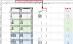
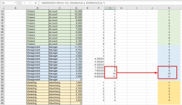
The reason for using the condition greater than or equal to 0.5 is:
I hope you are doing well. I've used the ROUNDUP and ROUND formulas to avoid the decimals in rank. Where numbers are rounded up if the decimal values are less than 0.5, or rounded and added +1 to the next integer if they are equal to or greater than 0.5. You can change the condition based on your data.
Formula : =IFERROR(IF(F5-INT(F5)>=0.8, ROUND(F5,0)+1, ROUNDUP(F5,0)),"")

The reason for using the condition greater than or equal to 0.5 is:

Attachments
Dear Jululian,
I hope you are doing well. I've used the ROUNDUP and ROUND formulas to avoid the decimals in rank. Where numbers are rounded up if the decimal values are less than 0.5, or rounded and added +1 to the next integer if they are equal to or greater than 0.5. You can change the condition based on your data.
Formula : =IFERROR(IF(F5-INT(F5)>=0.8, ROUND(F5,0)+1, ROUNDUP(F5,0)),"")
View attachment 1280
The reason for using the condition greater than or equal to 0.5 is:
View attachment 1281
Many thanks for your reply and for your time |
may I kindly request that I need to fix my formula, not the helper column and thank you agian |
You can use this formula : =IFERROR( IF(D5=0, "",IF(D5>0, IF( SUMPRODUCT(($B$5:$B$44=B5)*($C$5:$C$44=C5),(D5<=$D$5:$D$44)/COUNTIF($D$5:$D$44,$D$5:$D$44))-INT(SUMPRODUCT(($B$5:$B$44=B5)*($C$5:$C$44=C5),(D5<=$D$5:$D$44)/COUNTIF($D$5:$D$44,$D$5:$D$44)))>=0.8,ROUND(SUMPRODUCT(($B$5:$B$44=B5)*($C$5:$C$44=C5),(D5<=$D$5:$D$44)/COUNTIF($D$5:$D$44,$D$5:$D$44)),0)+1,ROUNDUP(SUMPRODUCT(($B$5:$B$44=B5)*($C$5:$C$44=C5),(D5<=$D$5:$D$44)/COUNTIF($D$5:$D$44,$D$5:$D$44)),0)), "" ) ), "")
To avoid a lengthy formula I used the previous formula.
If you are an advanced Excel user you can follow this formula too: =IFERROR(IF(D5=0,"",LET(sumProd,SUMPRODUCT(($B$5:$B$44=B5)*($C$5:$C$44=C5),(D5<=$D$5:$D$44)/COUNTIF($D$5:$D$44,$D$5:$D$44)),IF(sumProd-INT(sumProd)>=0.8,ROUND(sumProd,0)+1,ROUNDUP(sumProd,0)))),"")
Attachments
i am very sorry the formula is not working properly I attached the sheet for your kind reviewYou can use this formula : =IFERROR( IF(D5=0, "",IF(D5>0, IF( SUMPRODUCT(($B$5:$B$44=B5)*($C$5:$C$44=C5),(D5<=$D$5:$D$44)/COUNTIF($D$5:$D$44,$D$5:$D$44))-INT(SUMPRODUCT(($B$5:$B$44=B5)*($C$5:$C$44=C5),(D5<=$D$5:$D$44)/COUNTIF($D$5:$D$44,$D$5:$D$44)))>=0.8,ROUND(SUMPRODUCT(($B$5:$B$44=B5)*($C$5:$C$44=C5),(D5<=$D$5:$D$44)/COUNTIF($D$5:$D$44,$D$5:$D$44)),0)+1,ROUNDUP(SUMPRODUCT(($B$5:$B$44=B5)*($C$5:$C$44=C5),(D5<=$D$5:$D$44)/COUNTIF($D$5:$D$44,$D$5:$D$44)),0)), "" ) ), "")
To avoid a lengthy formula I used the previous formula.
If you are an advanced Excel user you can follow this formula too: =IFERROR(IF(D5=0,"",LET(sumProd,SUMPRODUCT(($B$5:$B$44=B5)*($C$5:$C$44=C5),(D5<=$D$5:$D$44)/COUNTIF($D$5:$D$44,$D$5:$D$44)),IF(sumProd-INT(sumProd)>=0.8,ROUND(sumProd,0)+1,ROUNDUP(sumProd,0)))),"")
Hello Jululiani am very sorry the formula is not working properly I attached the sheet for your kind review
We have reviewed your dataset and found that developing a formula using Excel's built-in functions to find sales rank based on department and section would be time-consuming.
So, we recommend using an Excel VBA User-defined function to meet your expectations when calculating sales rank.
Follow these steps:
- Press Alt+F11 to open the VBE.
- Click on Insert followed by Module.
- Paste the following code in the Module and save it:
Code:Function SalesRank(rngDepartment As Range, rngSection As Range, rngSales As Range, rngCellRange As Range) As Variant Dim lastRow As Long Dim currentDept As String Dim currentSection As String Dim currentSales As Long Dim currentRank As Variant Dim i As Long lastRow = rngDepartment.Parent.Cells(rngDepartment.Parent.Rows.Count, rngDepartment.Column).End(xlUp).Row currentDept = rngDepartment.Cells(1).Value currentSection = rngSection.Cells(1).Value currentSales = rngSales.Cells(1).Value currentRank = 1 For i = 1 To lastRow If rngDepartment.Cells(i).Value <> currentDept Or rngSection.Cells(i).Value <> currentSection Then currentRank = 1 currentDept = rngDepartment.Cells(i).Value currentSection = rngSection.Cells(i).Value currentSales = rngSales.Cells(i).Value End If If rngSales.Cells(i).Value = 0 Then currentRank = "" Else If rngSales.Cells(i).Value < currentSales Then currentRank = currentRank + 1 End If End If currentSales = rngSales.Cells(i).Value If rngCellRange.Cells(1).Row = rngSales.Cells(i).Row And rngCellRange.Cells(1).Column = rngSales.Cells(i).Column Then SalesRank = currentRank Exit Function End If Next i SalesRank = currentRank End Function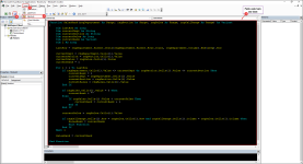
- Return to the sheet and select the desired cell.
- Apply the following formula:
=SalesRank($B$2:$B$162,$C$2:$C$162,$D$2:$D$162,D2) - Use the Fill Handle icon to copy the formula down.
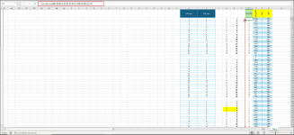
Regards
Lutfor Rahman Shimanto
Excel & VBA Developer
ExcelDemy
Attachments
many many thanks for a great solution and your response many thanks againHello Jululian
We have reviewed your dataset and found that developing a formula using Excel's built-in functions to find sales rank based on department and section would be time-consuming.
So, we recommend using an Excel VBA User-defined function to meet your expectations when calculating sales rank.
Follow these steps:
I am attaching the solution workbook for better understanding. I hope the User-defined function will help you; good luck.
- Press Alt+F11 to open the VBE.
- Click on Insert followed by Module.
- Paste the following code in the Module and save it:
View attachment 1289Code:Function SalesRank(rngDepartment As Range, rngSection As Range, rngSales As Range, rngCellRange As Range) As Variant Dim lastRow As Long Dim currentDept As String Dim currentSection As String Dim currentSales As Long Dim currentRank As Variant Dim i As Long lastRow = rngDepartment.Parent.Cells(rngDepartment.Parent.Rows.Count, rngDepartment.Column).End(xlUp).Row currentDept = rngDepartment.Cells(1).Value currentSection = rngSection.Cells(1).Value currentSales = rngSales.Cells(1).Value currentRank = 1 For i = 1 To lastRow If rngDepartment.Cells(i).Value <> currentDept Or rngSection.Cells(i).Value <> currentSection Then currentRank = 1 currentDept = rngDepartment.Cells(i).Value currentSection = rngSection.Cells(i).Value currentSales = rngSales.Cells(i).Value End If If rngSales.Cells(i).Value = 0 Then currentRank = "" Else If rngSales.Cells(i).Value < currentSales Then currentRank = currentRank + 1 End If End If currentSales = rngSales.Cells(i).Value If rngCellRange.Cells(1).Row = rngSales.Cells(i).Row And rngCellRange.Cells(1).Column = rngSales.Cells(i).Column Then SalesRank = currentRank Exit Function End If Next i SalesRank = currentRank End Function- Return to the sheet and select the desired cell.
- Apply the following formula:
- Use the Fill Handle icon to copy the formula down.
View attachment 1288
Regards
Lutfor Rahman Shimanto
Excel & VBA Developer
ExcelDemy
Dear Jululian, thanks for your kind words. You are most welcome.many many thanks for a great solution and your response many thanks again
