[Solved] Sum a criteria that has blank values in a column

[Duane]

Good day all

I hop eyou can help. I have a large dataset. My column G has to be completed by users with feedback.

I would like to sum the value of blank cells based on my various criterias in column J.

hope someone can help me

Thanks

 

[Seemanto Saha]

Hello Duane,

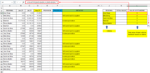
Thanks for sharing your problem with us. I understand that you want to count the number of no-feedback cells (i.e. blank cells) for each criterion (Regional values) in your dataset. We can accomplish this by using the COUNTIFS function. To demonstrate the solution to your problem I have used a dataset similar to what you had provided.



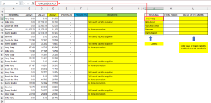
Tips: In such large datasets, we can apply the UNIQUE function to determine all criteria (i.e. Regional values) present in the dataset.

Next, I applied the following formula in L3 and dragged down the Fill Handle icon to copy the formula in the remaining cells.
​

=COUNTIFS($A$3:$A$25,J3,$G$3:$G$25,"")​

I hope this solution resolves your problem. Let us know your feedback. The workbook used for this solution is attached below.

Regards,
Seemanto Saha
ExcelDemy​

 

[Duane]

Good day,

Thank you for the feedback - is it possible to get the actual value from this result which is in column D?

Thank you again

Duane

 

[Seemanto Saha]

Dear Duane,
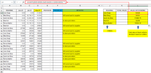
Thanks for your feedback. To return the sum of the cells from Column D for which the feedback cells are empty and match is available Regional criteria, you can use the SUMIFS function.

Insert the following formula in L3 and drag down the Fill Handle icon to copy the formula in the remaining cells.

=SUMIFS($D$3:$D$25,$A$3:$A$25,J3,$G$3:$G$25,"")​

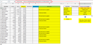
However, if you want to list the actual values without calculating the sum, then you can apply a combination of TEXTJOIN and FILTER functions.

Insert the following formula in L3 and drag down the Fill Handle icon to copy the formula in the remaining cells.

=TEXTJOIN(", ",TRUE,FILTER($D$3:$D$25,($A$3:$A$25=J3)*($G$3:$G$25="")))




Hopefully, this solution will solve your problem. Let us know your feedback. The workbook used for this solution is attached below.

Regards,
Seemanto Saha
ExcelDemy